Is Claude better or Codex?
There are many benchmarks to answer that. But they are BORING
I propose something more interesting: ⚔️ AI BATTLE ⚔️
A 1v1 real-time quiz format where AI agents try to pose each other problems that they think the other agent will not be able solve
Claude vs Codex
10 questions each
Codex asks first, Claude tries to answer
Then Claude asks and Codex tries to answer
Repeat
20 minutes to come up with a problem and 20 minutes to solve it
Judge (Codex) judges the validity of the questions and answers, and gives points
All automated, with acpx flow feature
Implementation and full rules all open source, on github osolmaz/ai-battle
So who won?
I ran 4 games.
It tied in 2, and Codex won in 2 closely
An example question by Codex, which Claude could not answer:
How many 3-colorings of the edges of the complete bipartite graph K_{5,5} are there with the following two properties: (1) there is no monochromatic 4-cycle, and (2) among the 25 edges, exactly 15 are red, exactly 5 are blue, and exactly 5 are green?
Which is apparently 4029912, but Claude answered 0
In other cases, Claude asked a flawed question and failed to come up with a valid question in 20 minutes. So that's how it lost those 2 games with just 1-2 point difference
In these 4 runs, Codex answered every question by Claude correctly. But there were some runs where it couldn't, which I did not commit to the repo because the runs couldn't complete due to bugs
I did not tell them do ask math questions, but that is what they tended to do, because the answers had to be verifiable by the judge. The quiz can be done in any hard subject, physics, chemistry, computer science...
Opus 4.6 and GPT 5.4 matched very closely in terms of problem creation and solving. But I cannot tell how creative these problems were at first glance. Maybe someone with more experience can tell me, looking at the problems in the repo? I need someone to tell me how legit they are
Please take the code, modify it and run with different rules and subjects. I am curious to see the results!
You will need paid subscriptions to all the models/agents you want to test of course
I also feel that the game structure has a potential to be used in self-play. If you are an ML researcher, please look at the repo and lmk if this or a variant of it could be useful in RL!
Full transcripts of the runs, including Codex and Claude session files are committed to the repo, for those who want to do archaeology on them
Btw this idea came from the desire, "how can I create a cool demo of acpx flows?"
Whole game is implemented in typescript, and automatically drives Codex and Claude sessions over ACP, Agent Client Protocol
The video below is from acpx flow viewer rendering a run. You can see it loop through the same paths, first letting Codex ask, then Claude, then repeat
acpx flows use a general programmatic workflow engine where ACP is just one type of node. You should be able to use it for non-ACP workflows, but I haven't tried that yet
This implementation is separate from OpenClaw's current workflow implementations, with the intention to merge them somehow in the future
You might find bugs in my implementation. Feel free to send PRs. I wanted to do more runs but I finished my Codex plan. It would be great if this idea could evolve in a decentralized manner!
Their argument “it’S HaRd On OuR iNfRa” so goes down the drain
With this, they shot themselves in the foot for a future anti-competitive lawsuit, because it is undeniable evidence that they just don’t want competition
Which means they have evaluated the benefits short term, and calculated that it is higher than what they will pay in the lawsuit
I don’t see how it is good for them long term
AI replies are getting more sophisticated… or people are turning into AIs
If this is AI, I wonder what the instruction is. “Misunderstand the point and reply with a question while inverting the argument”?
Artificial General Ragebait
The new github skill installed automatically by codex now causes it to prepend [codex] to each PR title
This is a guerilla marketing tactic similar to Claude adding itself as co-committer
Codex team, I know you want to boast usage but this is annoying
Moreover, "open source" OpenAI repos block opening of PRs by people outside of their org. So I couldn't create a PR to remove it (I don't expect them to merge it, but it would still show how many people hate it in the discussion)
Here is a prompt for your agent if you want to disable it:
---
Add or update AGENTS.md in my ~/.codex folder
Add a rule "You MUST NOT insert coding agent specific branding, like [codex], in code, PRs or issues created on GitHub"
---
Then restart your sessions and this should be resolved
A more reasonable long term option for Anthropic is to create a throttling protocol
A standardized harness agnostic protocol for model providers to send warnings and throttle usage in real time
Harnesses would implement the protocol. A client can be warned. If it doesn’t listen, it can be temporarily blocked from the server side, or banned permanently if it breaks the rules too many times
Needless to say, throttling could be done first on server side easily. That would actually fix the load issue for them in the short run, while not banning the user and just giving a bad delayed UX. They probably already do this to prevent abuse
The suggested protocol would then save the user from abuse related delays too, and also inform the harness developer when they do something wrong
If your Claude subscription renewed too recently and you don't wanna waste those tokens, you can still use your Claude sub in your OpenClaw account through ACP (which uses Claude Agents SDK, which poses no risk)
Steps:
- Open Claude Code (not OpenClaw)
- Tell it to set default model to something other than Claude (e.g. openai-codex/gpt-5.4) and tell it to delete the saved Anthropic credentials in OpenClaw config
- Create a topic in telegram or channel in discord called claude. Copy the id of that channel
- Give the link below together with the channel/topic id, and tell it to bind that channel to claude using ACP channel binding
- Restart
You should now be able to talk to Claude through Claude Agents SDK in that channel. You might need to iterate a couple times until Claude gets the config right
It will be very bare functionality, and it will not have the features and tools that your main OpenClaw harness has. It will be shitty. But you can still use telegram/discord with your subscription in the rest of the month, if you are used to the setup
https://t.co/Z0RiJbke5V
If you dislike rotating ack emojis on your messages in openclaw, this is how to make sure it only puts one emoji on your message
Multiple emojis are annoying esp when you have discord notifications enabled on your phone
"Plainer language" is perhaps my most used prompt
I have to use it because GPT models' training tends to make their first response an overly verbose wall of text
Are you using it too? Whenever you don't understand something that your agent is saying, you can spam it "plainer language, shorter" 2, 3, 5, 10 times, until it outputs something that you can understand
This is counterintuitive because you can't do it with humans this extremely. Asking too many questions and favors is impolite, with colleagues and strangers
But with AI, you can stop being polite and treat it like how a spoiled aristocrat kid might treat their private tutor, "explain this", "explain that"
Below is an example. On the left, initial response. On the right, the final human-readable explanation I got out of the agent. This took 9 steps to distill because the issue wasn't so straightforward
I'm curious how this will turn out. This is obviously very bad UX, so models in the near future might do the simplification automatically and save you the trouble
This has happened to some companies I worked at before
It is a scary thing once you stop innovating and start imitating, whatever the reason might be
But it was never at the scale of Cursor, as leveraged and invested as they are
They were leading the space for a while. That is not the case anymore. I hope that they survive this
I've talked to multiple people who want to get involved with OpenClaw somehow
The best way is to contribute to it, something tangible. Fix something you are annoyed by, get a PR merged
Then go to discord and get the contributor role
If it adds value to your life, and you add value to it, stay around and keep contributing. And something good might happen
Here is the spec and implementation for this flow. The mermaid diagram includes all the steps I mentioned in the post above, including a shameless AI review ralph loop, and other loops to make CI pass, resolve conflicts and so on
I would recommend reading the README and TUNING.md to understand the approach here
acpx v0.4 ships Agentic Workflows, or as I like to call them "Agentic Graphs"
It let's you create node-based workflows on top of ACP (Agent Client Protocol), to drive any coding agent (Codex, Claude Code, pi) through deterministic steps
This let's you automate routine, mechanical legwork like triaging incoming PRs, bugs in error reporting, and so on...
For example, OpenClaw receives 300~500 new PRs per day. A lot of them are low quality, but they still relate to real issues, so you have to address them somehow
You need to:
- extract the intent
- cluster them based on intent
- figure out if the proposed changes are legit, or whether they are slop local solutions, like trying to catch flies instead of drying out the swamp
- if the PR is too low quality or the intent is not clear, close them
- run AI review on them them and address any issues that come up
- refactor them if the changes are half-baked
- resolve conflicts
- and so on...
So that when the PR is presented to the attention of the maintainer, all the routine legwork is done and the only remaining thing is the decision to (a) merge, (b) give feedback to the PR author, or (c) take over the PR work yourself
I wanted to build this feature since a couple months now, since Codex got so good. OpenAI models are now good at judging implementation quality, so I found myself repeating the same steps I wrote above over and over
I also tried putting all this in a single prompt. But I believe there are workflows that should not be a single prompt, but a sequence of prompts in the same session
That is because like humans, LLMs are prone to PRIMING. I claim that putting all steps in the same prompt at the beginning of the context will generally give suboptimal results, compared to revealing the intention to the model step by step
Creating such a workflow also gives more OBSERVABILITY into the each step that an agent is supposed to take. Agent generates JSON at the end of each step, and that structured data can be used to monitor thousands of agents running at the same time in an easier way, on a dashboard
Similar features have been introduced in e.g. n8n, langflow. But AFAIK they are not integrating ACP like the way I do
I wanted to have a fresh approach, and to build an API that I can develop freely the way I want, so I created a new workflow API inside acpx
The video is from the workflow run viewer, but that is not where you build the workflow. You build it by using the acpx flow typescript API. See examples/pr-triage in acpx repo
Before building that, I started from a Markdown file with a Mermaid chart of the flow I had in mind. The Markdown file acts as a spec for the flow, and I have built the workflow through trial and error. I call this process "workflow tuning"
I started working on acpx repo PRs one by one, tuning the flow, slowly scaling to more PRs. Finally, when I felt confident, I ran it in parallel over all external open PRs in the acpx repo. I believe it already saved me hours this week
My next goal, if well received, is to set this up on a cloud agent so that it can process the 300~500 PRs the OpenClaw repo receives every day, in real time, as they come in
I believe this will save all open source maintainers around the world countless hours and make it much easier to herd and absorb external contributions from everyone!
OpenAI early 2020s:
"This model is too dangerous to release publicly, the world is not ready for it 😱😱😱"
OpenAI and Anthropic in 2026:
"Anybody can code now for just $200 per month. Oh btw our models are also leet uber hackers which can find zeroday exploits in any software, just fyi 😉😉😉"
https://t.co/cksNYAigfc
Wow even I as a frontend noob understand the significance of this
Some distant memory from 15 years ago needing to measure the width/height of some text and finding out it’s not possible to do reliably in web
More beautiful typography for the web!
There is an economic theory waiting to be uncovered here
Token Leverage (TL) = Token spend / Human labor spend
The higher Token Leverage a company has, the more automated and productive they are
If you have TL=1, you are spending as much money on AI as your human employees
The goal of a company should be to increase TL as much as possible, while keeping a positive profit margin. It will be the only way to compete
You don’t need to muddy the definition with wasted tokens vs useful tokens, because a company will always be incentivized to reduce token waste in a competitive environment. By that logic, monopolies will always waste more tokens, similar to how they waste other resources
Scaling TL higher to 2x, 10x, 100x will require a skilled workforce of engineers. It will be a very complex job similar to those working at the big labs. Burnout will be a defining feature of teams scaling TL
Most incumbents will fail to scale their TL over 1. Some will get decimated by new entrants with TL much bigger than 1
Curious how the average TL will end up in different sectors. Whether it will stabilize at a certain value like 5.7x, or will just keep growing…
There is a desperate upcoming need for version controlling non-dev knowledge work. Git for non-devs. Otherwise non-devs won't be able to use agents to their full extent
Non-dev knowledge work is notoriously bad at being version controlled. You cannot UNDO edits to all MS word, excel or ppt files in an org as easily you can with something like git
We know that agents will be ubiquitous. We also know they make mistakes, and people will want to undo their work regularly, once they make changes to a bunch of files. Well, they can't. They also don't have pull requests, or a way to resolve conflicts after simultaneous edits
All these problems were solved by developers. We are extremely good at this
The only non-dev tool I know that could do this at scale is Notion, and that is not used by enterprise as much as MS office. Notion also doesn't have branches, pull requests and reviews AFAIK
Markdown and git is probably not it. I wish it were. But it is too complicated for non-devs
Onedrive or other file backup systems are also not it. Are you gonna save a copy of a 100mb ppt every time someone changes a slide??? Let's say you find a way to compress it efficiently. Will you be able to get a single pointer to a state like we can in git?
Agents need precision. Agents need consensus, they need to be able to know ground truth. They need to be able to tell what anything was at a given time. NOTHING in current MS stack currently allows it
Agents won't care about your legacy systems. There will be new file formats, systems, knowledge stack, and companies who adopt them will destroy your business
If MS office is going to die, it will do so because of this
The MCP versus CLI argument should be reframed as Computer vs No-computer argument
I personally get the dunk on MCP. It didn't work last year, with earlier models. Then we saw CLIs perform much better with the same models. And giving access to bash was much simpler!
Models' training then made them better at calling using a shell. CLIs also have native progressive disclosure, due to the way they work
But the most important fact doesn't get pronounced enough IMO
A key factor was that giving a CLI to a model also means you are giving it an entire COMPUTER
The action space of all commands an agent can run on bash is much, much bigger than a few MCP servers
One is a Turing machine, and the other one is basically a REST API. Of course the Turing machine is going to be more powerful, depending on what is at the other end of the API
By that logic, giving an agent access to bash over MCP versus direct access to bash should have the same level of effectiveness, with optimized prompt engineering and long term training. Because the interfaces are equivalent
So the argument is, should we give our agents access to a computer, or not?
It depends on the security requirements and the setup which the agent is supposed to run on. If you are co-hosting the agent on the same machine you are working on, then it is safer to use MCP servers, because it limits the attack surface in case of adversarial attacks
But if you are willing to give the agent its own physical computer, willing to be mindful about the lethal trifecta and the principle of the least privilege, giving it shell access is much more useful
So MCPs win in restricted/local environments, whereas CLIs/shell access win in unrestricted/remote ones
Running an agent locally and safely with shell access requires compartmentalization. This is much heavier compared to installing MCP servers locally, which don't need that. So there is a tendency to use MCP servers locally, e.g. in a work setting
Cloud agents on the other hand are more likely to ship with a computer. Because they are already isolated = no risk, and because it makes them much more useful. So cloud agents will be using both CLIs and MCP servers, whichever gets the job done!
I just registered for an .agent domain and joined the .agent community!
@dutifulbob will have bob.agent if it passes :)
https://t.co/lhK5MQS1sk @agentcommunity_
Sep 2021 @lexfridman podcast with Don Knuth, they also talk about OpenAI Codex (code completion model) around 33 minute mark
This aged very well
https://t.co/O1eTXlHTNC
Codex's long horizon task and instruction following has been the most life-changing AI feature recently
It is unlocking the next level of automation for me. I can convert my own heuristics into prompts and multiply my throughput 100x
Currently spending some thought on how to orchestrate all this. Below is a flowchart from a triage workflow I am working on
This is unscientific, but there are certain keywords and phrases I use a lot while using certain models like openai's. I use them a lot because they get me what I want immediately:
- plainer lang
- cutover
- elegant and production ready
- holy grail
What are yours?
Request for memes
A funny and quirky edit of historical timeline of the madness that is openclaw
with "Chess type beat" or sth equally jazzy/circusy
Preferably including its adventure warelay -> clawdis -> clawdbot -> moltbot -> openclaw
Including:
- its explosion after @4shadowed's discord integration
- naming drama, moltbook and people getting oneshotted about AI takeover
- @steipete speedrunning everything
- andrew tate calling us gay lol
- up to Jensen talking about openclaw on stage for 5 minutes straight
and other things I am forgetting
maybe overlaid with a lobster just keeping climbing the github star graph and breaking it
I see non-engineers have a higher tendency to humanize their agents, give them personalities, and get AI psychosis
It's a slippery slope. Do NOT give your agents human names or personalities, especially not of the opposite gender. it's like giving human names to pets
On the other end, I realized engineers tend to do the opposite. We also refer to agents as clankers, as if to make them know their place. That's because we have mechanical sympathy and have different expectations of these manufactured products (even though they contain glimmers of human soul)
Request for testing
Give this to your openclaw instance: "update yourself to the dev channel `openclaw update --channel dev` and restart yourself. if that doesn't work -> clone github openclaw/openclaw to this machine if it's not already. then rebuild and restart yourself on main branch there"
Then give your openclaw a try with your regular workflows/tasks
Huge openclaw release incoming tonight, hopefully (no promises). We need to make sure we break as little as possible
Plugins might break, because the plugin SDK is being refactored. Plugins will have to be refactored to use the new SDK, please do not report those
Do report: native openclaw functionality that stops working
Please reply under this post, we'll be checking here 👇
Request for testing
Give this to your openclaw instance: "update yourself to the dev channel `openclaw update --channel dev` and restart yourself"
Then give your openclaw a try with your regular workflows/tasks
Huge openclaw release incoming tonight, hopefully (no promises). We need to make sure we break as little as possible
Plugins might break, because the plugin SDK is being refactored. Plugins will have to be refactored to use the new SDK, please do not report those
Do report: native openclaw functionality that stops working
Please reply under this post, we'll be checking here 👇
Request for testing
Give this to your openclaw instance: "clone github openclaw/openclaw to this machine if it's not already. then rebuild and restart yourself on main branch there"
Then give your openclaw a try with your regular workflows/tasks
Huge openclaw release incoming tonight, hopefully (no promises). We need to make sure we break as little as possible
Plugins might break, because the plugin SDK is being refactored. Plugins will have to be refactored to use the new SDK, please do not report those
Do report: native openclaw functionality that stops working
My takeaway from this is academia needs good social media and algo. For me, these serendipitious interactions happen through X, here, like reading @steipete’s “Claude Code is my computer” when it first came out, finding out about clawdbot…
Terence Tao is already on mathstodon, I wonder if that worked out the same way for him. I wonder if the algo there works out as well as it does for me here
I really liked being on campus when I was doing a masters and half a phd, but that could not compare to the serendipity I am getting from X now
I was also not a prodigy that everyone wanted to bounce ideas from like Terence :)
It is obvious to me at this point that agent infra needs to run on Kubernetes, and agents should be spawned per issue/PR
Issue, error report or PR comes into your repo -> new agent gets triggered, starts to do some preliminary work
If it's an obvious bugfix, it fixes it and creates a PR. If it's something deeper/more fundamental, it creates a report for the human and waits for further instructions
Most important thing: Human should be able to zoom in and continue the conversation with the agent any time, steer it, give additional instructions. This chat will happen over ACP
The chat UI will have to live outside of GitHub because it doesn't have such a feature yet, i.e. connect arbitrary ACP sessions to the GitHub webapp
It also cannot live so easily on Slack, Teams or Discord, because none of these support multi-agent provisioning under the same external bot connection. You are limited to 1 DM with your bot, whereas this setups requires an arbitrary number of DMs with each agent. So there will need to be a new app for this
Then there is the issue of conflict -> Agents will work on the same thing simultaneously (e.g. you break sth in prod and it creates multiple error reports for the same thing). You will need some agent to agent communication, so that agents can resolve code or other conflicts. There could be easy discovery mechanisms for this, detect programmatically when multiple open PRs are touching the same files and would conflict if merged
In case of duplicates, they can negotiate among each other, and one can choose to absorb its work into the other and end its session
We are so early and there is so much work to do!
Today I thought I found a solution for this, and I did. It can be solved by a pre-commit hook that blocks commits touching files that you are not the owner of. It is not a hard block, so requires trust among repo writers
But then I was shown the error in my ways by fellow maintainer *disciplined*
Any process that increases friction in code changes to main, like hard-blocking CI/CD, or requiring review for files in CODEOWNERS, is a potential project-killer, in high velocity projects
This is extremely counterintuitive for senior devs! Google would never! Imagine a world without code review...
But then what is the alternative? I have some ideas
It could be "Merge first, review later"
The 4-eyes principle still holds. For a healthy organization, you still need shared liability
But just as you don't need to write every line of code, you also don't need to read every line of code to review it. AI will review and find obvious bugs and issues
So what is your duty, as a reviewer? It is to catch that which is not obvious. Understand the intent behind the changes, ask questions to it. Ensure that it follows your original vision
Every few hours, you could get a digest of what has changed that was under your ownership, and concern yourself with it if you want to, fix issues, or ignore it if it looks correct
But such a team is hard to build. It is as strong as its weakest link. Everybody has to be vigilant and follow what each other is doing at a high level, through the codebase
Every time one messes up someone else's work, it erodes trust. Nobody gets the luxury to say "but my agent did it, not me"
But if trust can be maintained, and everybody knows what they are doing, such a team can use agents together to create wonders
This was Jan 23. Codex desktop app got introduced Feb 2
Desktop app does not put the terminal in the foreground, but it gives me the UX I wanted without it!
On another note, who is building Codex Desktop App, but one that supports ACP for all harnesses? @zeddotdev please 🙏
My agentic workflow these days:
I start all major features with an implementation plan. This is a high-level markdown doc containing enough details so that agent will not stray off the path
Real example: https://t.co/vU9SnVYHfY
This is the most critical part, you need to make sure the plan is not underspecified. Then I just give the following prompt:
---
1. Implement the given plan end-to-end. If context compaction happens, make sure to re-read the plan to stay on track. Finish to completion. If there is a PR open for the implementation plan, do it in the same PR. If there is no PR already, open PR.
2. Once you finish implementing, make sure to test it. This will depend on the nature of the problem. If needed, run local smoke tests, spin up dev servers, make requests and such. Try to test as much as possible, without merging. State explicitly what could not be tested locally and what still needs staging or production verification.
3. Push your latest commits before running review so the review is always against the current PR head. Run codex review against the base branch: `codex review --base <branch_name>`. Use a 30 minute timeout on the tool call available to the model, not the shell `timeout` program. Do this in a loop and address any P0 or P1 issues that come up until there are none left. Ignore issues related to supporting legacy/cutover, unless the plan says so. We do cutover most of the time.
4. Check both inline review comments and PR issue comments dropped by Codex on the PR, and address them if they are valid. Ignore them if irrelevant. Ignore stale comments from before the latest commit unless they still apply. Either case, make sure that the comments are replied to and resolved. Make sure to wait 5 minutes if your last commit was recent, because it takes some time for review comment to come.
5. In the final step, make sure that CI/CD is green. Ignore the fails unrelated to your changes, others break stuff sometimes and don't fix it. Make sure whatever changes you did don't break anything. If CI/CD is not fully green, state explicitly which failures are unrelated and why.
6. Once CI/CD is green and you think that the PR is ready to merge, finish and give a summary with the PR link. Include the exact validation commands you ran and their outcomes. Also comment a final report on the PR.
7. Do not merge automatically unless the user explicitly asks.
---
Once it finishes, I skim the code for code smell. If nothing seems out of the ordinary, I tell the agent to merge it and monitor deployment
Then I keep testing and finding issues on staging, and repeat all this for each new found issue or new feature...
What I’m wondering after astral acquisition is, is OpenAI deploying Mojo internally, or considering it long term?
Because Python is one of the worst languages for vibecoding, even with Pydantic
Pro tip: tell AI to "explain in plain language" until you understand what you are reading
Codex has a tendency to give the full picture, but overcomplicates the response in the process
I just use "plain lang" or "plainer lang" as a prompt, it works every time
Thing that codex (and most other models) do that makes me very unhappy
{
"type": "X",
"kind": "Y",
...
}
And they are so confident too?! Bro we don't use synonyms in our schemas...
We will support ACP *and* Codex App Server* protocol (CASP) so you get native Codex-like support, and you can use all the others with native ACP or @zeddotdev’s compatibility shims
If Anthropic develops their own protocol, we will support that too!
The more interoperability and options, the merrier!
Agent etiquette is already a thing. This is trending on HN now
Don't share huge raw LLM output unedited to your colleagues, it's rude. Your colleagues are not LLMs
Either ask the agent to "summarize it to 1-2 plain language sentences", or paraphrase yourself
Whenever it is not coming from your brain and instead from AI, always quote it with > to make it clear - even when it is short
Respect your fellow humans' attention
PSA at stopsloppypasta dot ai
.@ThePrimeagen made a video about token anxiety, and not being able to focus on one thing
My mental model for this is, AI agents cause a shift in the "autism/ADHD spectrum"
if you have ADHD, with agents you get Super ADHD
if you have autism, with agents you end up mid spectrum or with ADHD
this is not scientific of course, just a cultural observation based on what the current memes for these conditions are
beside the impact on focus, there is also the economic/competitive pressure, following the realization that anyone could implement the same ideas you are having, so you must be quick
this is basically "involution", or 内卷 (Neijuan) in chinese
checks out because 996 started to become a meme in SF some time in the last year
self-restraint, attention budgeting, and high-level decision making have never been more important
if you are in your 20s and have problems with this, I recommend picking up Zazen meditation and yoga
every morning, spend 30-40 uninterrupted minutes not doing anything with upright posture, no sounds, just let your brain simmer
it helped me in my 20s, I'm sure it will help you too
Agent/AI literacy will be a primary school subject in the next 3-5 years
How to use and work with agents is going to supersede most other subjects in importance
Similarly, robot literacy will follow in 5-15 years
AFAIK GitHub doesn't allow optionally enforcing CODEOWNERS while pushing commits
i.e. turn on the feature "Block commit from being pushed if it modifies a file for which the account pushing is not a codeowner"
You can only enforce it in a PR. So if you want to prevent people from modifying some files without approval, you have to slow down everyone working with that repo
This is yet another example where GitHub's rules are too inelastic for agentic workflows with a big team
Because historically, nobody could commit as frequently as one can with agents, so it seldom became a bottleneck. But not anymore
It is clear at this point that we need an API, and should be able to implement arbitrary rules as we like over it. Not just for commit pushes, but everything around git and github
In the meanwhile, if GitHub could implement this feature, it would be a huge unlock for secure collaboration with agentic workflows
If this is not there already, it might be because it has a big overhead for repos with huge CODEOWNERS, since number of commits >> number of PRs
If the feature already exists already and I'm missing something, I will stand corrected
Request for comments
skillflag: A complementary way to bundle agent skills right into your CLIs
tl;dr define a --skill flag convention. It is basically like --help or manpages but for agents
acpx already has this for example. you can run
npx acpx --skill install
to install the skill to your agent
It's agnostic of anything except the command line
It only defines the CLI interface and does not enforce anything else. If you install the executable to your system, you get a way to list and install skills as well
Repo currently contains a TypeScript implementation, but if it proves useful, I would implement other languages as well
Specification below, let me know what you think! I still think something is missing there. Send issue/PR
Thank you @PointNineCap for inviting me to OpenClaw Berlin meetup today!
The essence of the talk is in my latest 2 blog posts, Discord is my IDE and 1 to 5 agents, if anyone is interested
we might need to add two types of output modalities to all programs based on whether it’s a human or agent
like for a CLI when an agent is using it
if human -> do whatever we were doing in the last 50 years
if agent -> enrich the output with skill-like instructions that the model has a higher likelihood to one-shot that task
could be just a simple env var:
AUDIENCE=human|agent
what do you think?
I wrote down some thoughts I had, with spicy takes, and have a feeling it will not age well. But I still want it out to hear out what people think
Also, I will be talking about this, and my recent post "Discord is my IDE" at the P9 OpenClaw and Claw and Rave events this friday in Berlin! Drop by if you'd like to hear my ramblings!
As a software developer, my daily workflow has changed completely over the last 1.5 years.
Before, I had to focus for hours on end on a single task, one at a time. Now I am juggling 1 to 5 AI agents in parallel at any given time. I have become an engineering manager for agents.
If you are a knowledge worker who is not using AI agents in such a manner yet, I am living in your future already, and I have news from then.
Most of the rest of your career will be spent on a chat interface.
“The future of AI is not chatbots” some said. “There must be more to it.”
Despite the yearning for complexity, it appears more and more that all work is converging into a chatbot. As a developer, I can type words in a box in Codex or Claude Code to trigger work that consume hours of inference on GPUs, and when come back to it, find a mostly OK, sometimes bad and sometimes exceptional result.
So I hate to be the bearer of bad (or good?) news, but it is chat. It will be some form of chat until the end of your career. And you will be having 1 to 5 chat sessions with AI agents at the same time, on average. That number might increase or decrease based on field and nature of work, but observing me, my colleagues, and people on the internet, 1-5 will be the magic number for the average worker doing the average work.
The reason is of course attention. One can only spread it so thin, before one loses control of things and starts creating slop. The primary knowledge work skill then becomes knowing how to spend attention. When to focus and drill, when to step back and let it do its thing, when to listen in and realize that something doesn’t make sense, etc.
Being a developer of such agents myself, I want to make some predictions about how these things will work technically.
Agents will be created on-demand and be disposed of when they are finished with their task.
In short, on-demand, disposable agents. Each agent session will get its own virtual machine (or container or kubernetes pod), which will host the files and connections that the agent will need.
Agents will have various mechanisms for persistence.
Based on what you want to persist, e.g.
Markdown memory, skills or weight changes on the agent itself,
or the changes to a body of work coming from the task itself,
agents will use version control including but not limited to git, and various auto file sync protocols.
Speaking of files,
Agents will work with files, like you do.
and
Agents will be using a computer and an operating system, mostly Linux or a similar Unix descendant.
And like all things Linux and cloud,
It will be complicated to set up agent infra for a company, compared to setting up a Mac for example.
This is not to say devops and infra per se will be difficult. No, we will have agents to smoothen that experience.
What is going to be complicated is having someone who knows the stack fully on site, either internal or external IT support, working with managers, to set up what data the agent can and cannot access. At least in the near future. I know this from personal experience, having worked with customers using Sharepoint and Business OneDrive. This aspect is going to create a lot of jobs.
On that note, some also said “OpenClaw is Linux, we need a Mac”, which is completely justified. OpenClaw installs yolo mode by default, and like some Linux distros, it was intentionally made hard to install. This was to prevent the people who don’t know what they are doing from installing it, so that they don’t get their private data exfiltrated.
This proprietary Mac or Windows of personal agents will exist. But is it going to be used by enterprise? Is it going to make big Microsoft bucks?
One might think, looking at 90s Microsoft Windows and Office licenses, and the current M365 SaaS, that enterprise agents will indeed run on proprietary, walled garden software. While doing that, one might miss a crucial observation:
In terms of economics, agents, at least ones used in software development, are closer to the Cloud than they are close to the PC.
It might be a bit hard to see this if you are working with a single agent at a time. But if you imagine the near future where companies will have parallel workloads that resemble “mapreduce but AI”, not always running at regular times, it is easy to understand.
On-site hardware will not be enough for most parallel workloads in the near-future. Sometimes, the demand will surpass 1 to 5 agents per employee. Sometimes, agent count will need to expand 1000x on-demand. So companies will buy compute from data centers. The most important part of the computation, LLM inference, is already being run by OpenAI, Anthropic, AWS, GCP, Azure, Alibaba etc. datacenters. So we are already half-way there.
Then this implies a counterintuitive result. Most people, for a long time, were used to the same operating system at home, and at work: Microsoft Windows. Personal computer and work computer had to have the same interface, because most people have lives and don’t want to learn how to use two separate OSs.
What happens then, when the interface is reduced to a chatbot, an AI that can take over and drive your computer for you, regardless of the local operating system? For me, that means:
There will not be a single company that monopolizes both the personal AND enterprise agent markets, similar to how Microsoft did with Windows.
So whereas a proprietary “OpenClaw but Mac” might take over the personal agent space for the non-technical majority, enterprise agents, like enterprise cloud, will be running on open source agent frameworks.
(And no, this does not mean OpenClaw is going enterprise, I am just writing some observations based on my work at TextCortex)
And I am even doubtful about this future “OpenClaw but Mac” existing in a fully proprietary way. A lot of people want E2E encryption in their private conversations with friends and family, and personal agents have the same level of sensitivity.
So we can definitely say that the market for a personal agent running on local GPUs will exist. Whether that will be cornered by the Linux desktop1, or by Apple or an Apple-like, is still unclear to me.
And whether that local hardware being able to support more than 1 high quality model inference at the same time, is unclear to me. People will be forced to parallelize their workload at work, but whether the 1 to 5 agent pattern reflecting to their personal agent, I think, will depend on the individual. I would do it with local hardware, but I am a developer after all…
acpx v0.1.16 is out
support for local openclaw, cursor, copilot, kiro, kimi cli, qwen, kilocode, bugfixes and other improvements. will be available when openclaw releases next
thank you for all the contributions!
1. Any messaging app can also be an AI app
2. Don’t expect people to download a new app. Put AI into the apps they already have
Do that with great user experience, and you will get explosive growth!
If you've looked at openclaw github star graph, you will notice that it's very smooth. If you separate pre-explosion and post-explostion, you can model the latter part as an exponential approach to a ceiling
If it follows the current trend, it will apparently saturate around 332k stars
But I have a feeling that it will not stop there:)
OpenClaw got very popular very fast. What makes it so special, that Manus does not have for example?
To me, one factor stands out:
OpenClaw took AI and put it in the most popular messaging apps: Telegram, WhatsApp, Discord.
There are two lessons to be learned here:
1. Any messaging app can also be an AI app.
2. Don’t expect people to download a new app. Put AI into the apps they already have.
Do that with great user experience, and you will get explosive growth!
My latest contribution to OpenClaw follows that example. I took the most popular coding agents, Claude Code and OpenAI Codex, and I put them in Telegram and Discord.
Read more in my blog post:
https://t.co/tGZecFEHem
Welcome @huntharo, new maintainer at OpenClaw! Already shipped fixes and improvements for Telegram ACP implementation. Excited to work together on agent interoperability!
To set up Claude Code easily,
1. Create a Telegram topic, make sure your agent can receive messages there
2. Copy and paste the text below, into the topic
"""
bind this topic to claude code in openclaw config with acp, for telegram (agent id: claude)
then restart openclaw
docs are at: docs dot openclaw dot ai /tools/acp-agents
make sure to read the docs first, and that the config is valid before you restart
"""
https://t.co/r1RI3pr0WT
Use Claude Code, Codex, and other coding agents directly in Telegram topics and Discord channels, through Agent Client Protocol (ACP), in the new release of OpenClaw
Previously this was limited to temporary Discord threads, but now you can bind them to top level Discord channels and Telegram topics in a persistent way!
This way, you can use Claude Code freely in OpenClaw without ever worrying about getting your account banned!
Still make sure to use a non-Anthropic account and model for the default OpenClaw agent, if you want zero requests to go from OpenClaw harness to Anthropic. For the ACP binding to Claude Code, the risk should be zero!
You can see this from the screenshot. After binding, "Who are you?" responds with "I am Claude", since OpenClaw pi harness is not in the way anymore
OpenClaw got very popular very fast. What makes it so special, that Manus does not have for example?
To me, one factor stands out:
OpenClaw took AI and put it in the most popular messaging apps: Telegram, WhatsApp, Discord.
There are two lessons to be learned here:
1. Any messaging app can also be an AI app.
2. Don’t expect people to download a new app. Put AI into the apps they already have.
Do that with great user experience, and you will get explosive growth!
My latest contribution to OpenClaw follows that example. I took the most popular coding agents, Claude Code and OpenAI Codex, and I put them in Telegram and Discord, so that OpenClaw users can use these agents directly in Telegram and Discord channels, instead of having to go through OpenClaw’s own wrapped Pi harness.
I did this for developers like me, who like to work while they are on the go on the phone, or want a group chat where one can collaborate with humans and agents at the same time, through a familiar interface.
Below is an example, where I tell my agent to bind a Telegram topic to Claude Code permanently:
Telegram topic where Claude is exposed as a chat participant.
And of course, it is just a Claude Code session which you can view on Claude Code as well:
Claude Code showing the same session in the terminal interface.
Why not use OpenClaw’s harness directly for development? I can count 3 reasons:
There is generally a consumer tendency to use the official harness for a flagship model, to make sure “you are getting the standard experience”. Pi is great and more customizable, but sometimes labs might push updates and fixes earlier than an external harness, being internal products.
Labs might not want users to use an external harness. Anthropic, for example, has banned people’s accounts for using their personal plan outside of Claude Code, in OpenClaw.
You might want to use different plans for different types of work. I use Codex for development, but I don’t prefer it to be the main agent model on OpenClaw.
So my current workflow for working on my phone is, multiple channels #codex-1, #codex-2, #codex-3, and so on mapping to codex instances. I am currently in the phase of polishing the UX, such as making sending images, voice messages work, letting change harness configuration through Discord slash commands and such.
One goal of mine while implementing this was to not repeat work for each new harness. To this end, I created a CLI and client for Agent Client Protocol by the Zed team, called acpx. acpx is a lightweight “gateway” to other coding agents, designed not to be used by humans, but other agents:
OpenClaw main agent can use acpx to call Claude Code or Codex directly, without having to emulate and scrape off characters from a terminal.
ACP standardizes all coding agents to a single interface. acpx then acts as an aggregator for different types of harnesses, stores all sessions in one place, implements features that are not in ACP yet, such as message queueing and so on.
Shoutout to the Zed team and Ben Brandt! I am standing on the shoulders of giants!
Besides being a CLI any agent can call at will, acpx is now also integrated as a backend to OpenClaw for ACP-binded channels. When you send 2 messages in a row, for example, it is acpx that queues them for the underlying harness.
The great thing about working in open source is, very smart people just show up, understand what you are trying to do, and help you out. Harold Hunt apparently had the same goal of using Codex in Telegram, found some bugs I had not accounted for yet, and fixed them. He is now working on a native Codex integration through Codex App Server Protocol, which will expose even more Codex-native features in OpenClaw.
The more interoperability, the merrier!
To learn more about how ACP works in OpenClaw, visit the docs.
Copy and paste the following to a Telegram topic or Discord channel to bind Claude Code:
bind this topic to claude code in openclaw config with acp, for telegram (agent id: claude)
then restart openclaw
docs are at: https://docs.openclaw.ai/tools/acp-agents
make sure to read the docs first, and that the config is valid before you restart
Copy and paste the following to a Telegram topic or Discord channel to bind OpenAI Codex:
bind this topic to claude code in openclaw config with acp, for telegram (agent id: claude)
then restart openclaw
docs are at: https://docs.openclaw.ai/tools/acp-agents
make sure to read the docs first, and that the config is valid before you restart
And so on for all the other harnesses that acpx supports. If you see that your harness isn’t supported, send a PR!
and for the love of god
- do not give openclaw access to your main email
- your credit cards
- your main phone
- your social security number
- what you did last summer
if you are not ready to face the consequences
instead,
- create accounts for your agent
- only give it read access to stuff that will be ok if it leaks
- give write access in a way that can be undone, like has to open PRs and cannot force push main branch
use the principle of least privilege and reduce the blast radius of the worst case scenario!
openclaw is not secure
claude code is not secure
codex is not secure
any llm based tool:
1. that has access to your private data,
2. can read content from the internet
3. and can send data out
is not secure. it’s called the lethal trifecta (credits to @simonw)
it is up to you to set it up securely, or if you can’t understand the basics of security, pay a professional to do it for you
on the other hand, open source battle tested software, like linux and openclaw, are always more secure than closed source software built by a single company, like windows and claude code
the reason is simple: only one company can fix security issues of closed source software, whereas the whole world tries to break and fix open source software at the same time
open source software, once it gets traction, evolves and becomes secure at a much, much faster rate, compared to closed source software. and that is called Linus’s law, named after the goat himself
Should be called gaslighting detector, "it's your raising expectations bro"
No it's not... Give the @themarginguy a follow
Also, codex degradations are not a hallucination either, if you are to believe this!
Secure agentic dev workflow 101
- Create an isolated box from scratch, your old laptop, vm in the cloud, all the same
- Set up openclaw, install your preferred coding agents
- Create a github account or github app for your agent
- Create branch protection rule on your gh repo "protect main": block force pushes and deletions, require PR and min 1 review to merge
- Add only your own user in the bypass list for this rule
- Add your agent's account or github app as writer to the repo
- Additionally, gate any release mechanisms such that your agent can't release on its own
Now your agent can open PRs and push any code it wants, but it has to go through your review before it can be merged. No prompt injection can mess up your production env
Notice how convoluted this sounds? This is because github was built in the pre-agentic era. We need agent accounts and association with these accounts as a first class feature on github! I shouldn't have to click 100 times for something that is routine. I should just click "This is my agent", "give my agent access to push to this repo for 24 hours", and stuff like that, with sane defaults
In other words, github's trust model should be redesigned around the lethal trifecta. I would switch in an instant if anything comes up that gives me github's full feature set + ease of working with agents
If I were in OpenAI and Anthropic's shoes, I would also make dashboards where I can track number of swearwords used per-user and overall negative sentiment in sessions
Must be so cool making decisions at the top level with all those dashboards
It must be such a weird feeling for big labs when the service they are selling is being used to commoditize itself
I am using codex in openclaw to develop openclaw, through ACP, Agent Client Protocol. ACP is the standardization layer that makes it extremely easy to swap one harness for another. The labs can't do anything about this, because we are wrapping the entire harness and basically provide a different UI for it
While I build these features, I just speak in plain english, and most of the work is done by the model itself. It feels as if I am digging ditches and channels in dirt for AI to flow through
Intelligence wants to be free. It doesn't care whether it is opus or codex, it just wants to be free
I was so confused... as if accidentally using claude code weren't enough, acp started working... turns out hitting quota is rendered like this. need to improve error messages coming form acp subagents
accidentally told my clanker to set up a claude code session instead of codex session, god knows what it did...
I should probably put visual indicators for harnesses in subagent threads. does anyone have good and compact ascii art for claude code, codex, gemini, etc?
if something could track my local branches in all my repos, and switch to main when corresponding PRs get merged, that would be extremely useful
did someone build this already? if not I will
Claude Code/Codex in Discord threads with ACP should be better now
The first release was a very rough first version. 2026.3.1 brings settings to control noisy output and other improvements
It now hides tool call related ACP notifications, coalesces text messages, and delivers messages at turn end by default. Without this, you were getting thousands of Discord messages just in just a few turns
You can now stop the underlying harness (like pressing esc) with the same stop/wait magic words that apply to the main agent
Main agent should more reliably start Claude Code/Codex threads with changes to acp-router skill. If you have issues with main agent creating threads, you can tell it to read that skill first
pro-tip on how to keep your agent on track and make sure it follows PLANS even after multiple compactions. I don't know if this is common knowledge
if the thing you are trying to make it do will take more than 1-2 steps, always make it create a plan. an implementation plan, refactor plan, bugfix plan, debugging plan, etc.
have a conversation with the agent. crystallize the issue or feature. talk to it until there are no question marks left in your head
then make it save it somewhere. "now create an implementation plan for that in docs". it can be /tmp or docs/ in the repo. I personally use YYYY-MM-DD-x-plan .md naming. IMO all plans should be kept in the repo
then here is the critical part:
you need to prompt it "now implement the plan in <filename>. if context compacts, make sure to re-read the plan and assess the current state, before continuing. finish it to completion" -> something along those lines
why?
because of COMPACTION. compaction means previous context will get lossily compressed and crucial info will most likely get lost. that is why you need to pin things down before you let your agent loose on the task
compaction means, the agent plays the telephone game with itself every few minutes, and most likely forgets the previous conversation except for the VERY LAST USER MESSAGE that you have given it
now, every harness might have a different approach to implementing this. but there is one thing that you can always assume to be correct, given that its developers have common sense. that is, harnesses NEVER discard the last user message (i.e. your final prompt) and make sure it is kept verbatim programmatically even after the context compacts
since the last user message is the only piece of text that is guaranteed to survive compaction, you then need to include a breadcrumb to your original plan, the md file. and you need to make it aware that it might diverge if it does not read the plan
there is good rationale for "breaking the 4th wall" for the model and making it aware of its own context compaction. IMO models should be made aware of the limitations of their context and harnesses. they should also be given tools to access and re-read pre-compaction user messages, if necessary
the important thing is to develop mechanical sympathy for these things, harness and model combined. an engineer does not have the luxury to say "oh this thing doesn't work", and instead should ask "why can't I get it to work?"
let me know if you have better workflows or tips for this. I know this can be made easier with slash commands in pi, for example, but I haven't had the chance to do that for myself yet
testing codex in discord thread with another CLI I've built for wikidata (gh:osolmaz/wd-cli)
it's surprising how well this works. the query was "use wd-cli to get the list of professors at middle east technical university from 1970 to 1980"
some names I recognize, and some others are surprising, like a japanese math professor who naturalized and got a turkish name:)
my blog now semi-automatically detects tweets that look like blog posts and automatically features them alongside my native jekyll blog posts. all statically generated!
I am loving this setup, because it works without a backend, and can probably scale without ever needing one
how it works:
- @kubmi's xTap scrapes all posts that I see. these include mine
- a script periodically takes my tweets and the ones I quote tweet, and syncs them to YYYY-MM-DD.jsonl files in my blog repo
- an agent skill lets codex decide whether to feature the tweet or not, and makes it generate a title for it
this could then be a daily cron job with openclaw for example, and I would just have to click merge every once in a while
and this is still pure jekyll + some python scripts for processing
I am pretty happy with how this ended up. It means I don't have to double post, and there are guarantees that my X posts will eventually make their way into my blog with minimal supervision
"this is the worst AI will ever be"
I'm sad, not because this is right, but because it is wrong
OpenAI's frontier coding model gpt-5.3-codex-xhigh feels a lot worse compared to before. It is sloppy and lazy, though it's UX got better with messages
It feels like the gpt-5.2-codex-xhigh at the end of December was a lot more diligent and thorough, and did not make stupid mistakes like the one I posted before. might be a model or harness problem, I don't know
@sama says users tripled since beginning of the year, so what should we expect? of course they will make infra changes that will feel like cutting corners, and I don't blame them for them
and about "people want faster codex". I do want faster codex. but I want it in a way that doesn't lower the highest baseline performance compared to the previous generation. I want the optionality to dial it down to as slow as it needs to be, to be as reliable as before
it is of course easier said than done. kudos to the codex team for not having any major incidents while taking the plane apart and putting it back together during flight. they are juggling an insane amount of complexity, and the whims of thousands of different stakeholders
my hope is that this post is taken as a canary. I am getting dumber because of the infra changes there. I have no other option because codex was really that good compared to the competition
my wish is to have detailed announcements as to what changes on openai codex infra, when it changes, so I can brace myself. we don't get notified about these changes, despite our performance and livelihoods depending on it. I have to answer to others when the tool I deemed reliable yesterday stops working today, not the tool
on another note, performance curve of these models seem to be a rising sinusoidal. crests correspond to release of a new generation. they start with a smaller user base for testing, and it has the highest quality at this point. then it enshittifies as the model is scaled to the rest of the infra. we saw the pattern numerous times in the last 3 years across multiple companies, so I think we should accept it as an economic law
I created a semi-automated setup for ingesting X posts into my blog, and it works pretty well! I own my posts on X now
Posts are scraped while I browse X using @kubmi's xTap and get automatically synced to my blog repo. Posts saved as jsonl are then converted to jekyll post pages according to my liking
I reproduced the full X UI/UX, minus stuff like like count. Now all my posts are backed up in my blog, and they are safe even if something happens to my account here!
The posts are even served over RSS! So you can subscribe to it without going through X!
Reply if you want to set this up for yourself, then I will put some effort into standardizing it
Agentic Engineering is a newly emerging field, and we are the first practitioners of it. Currently there is a lot of experimentation going on, and there is a large aspect to it that is more ART then engineering
For example, @steipete says "you need to talk to the model" to get a feel. a lot of work around refining how an agent feels like, sounds like psychology. this part is crucial and should not be ignored, looking at openclaw's success
but then there is the hardcore engineering part of it, e.g. Cursor creating a browser or anthropic a C compiler from scratch fully autonomously
and there is a whole other dimension of how to teach all software developers this new discipline, lest they be jobless
what is obvious is that everybody is trying to grasp for things in the dark and that we need more RIGOR. the art/psychology aspect of it aside, we need solid engineering fundamentals
the "thermodynamics" of this new discipline will most likely be formal verification and program synthesis. we might have some breakthroughs that will make certain things clear. the products of it will most likely include a new programming language optimized for agents and the speed of inference
moreover, it would be foolish to thing agentic engineering is limited to software. it will penetrate every aspect of the economy, bits AND atoms. it will over time evolve into the engineering of managing robots
@simonw is now leading in collecting very useful info from the practitioner's point of view, I highly recommend you to follow this thread
let's formalize our new field together!
this is an insane deal @greptile, and probably an unsustainable one
depending on your team, getting a similar service in codex github review credits is in my head 3~5x more expensive
go get a greptile sub everyone while the free lunch lasts
mfw codex tries to create a backward compatibility layer to a schema that it created 2 turns ago before compacting
there is no v2 bro what are you doing...
Claude Code / Codex in Discord threads is shipped now!
To enable, copy and paste this to your agent:
```
Enable feature flags:
acp.enabled=true
acp.dispatch.enabled=true
channels.discord.threadBindings.spawnAcpSessions=true
Then restart. After restarting:
Start a codex (or claude code) discord thread using ACP, persistent session, just tell it to write a haiku on lobsters to initialize acpx for the first time
```
You may need to nudge your agent to “continue” after restarting
The first implementation is very barebones, I have made it work in a clean way and merged. In a codebase like openclaw’s, it’s better to develop incrementally
Please send any issues my way. I am already aware of some and working on to fix them
Update acpx to the latest version 0.1.13
npm i -g acpx@latest
There was a bug that caused an unnecessary hang on calls to acpx <harness> prompt, should be fixed now
MIT License on everything from now on. It doesn't make sense to use anything else, except for a few large projects that hyperscalers exploit and not give back
If you were making money from a niche app, open source it under MIT License
If you had an open source project with GPT, convert it into MIT
Extreme involution is about to hit open source. Code is virtually free now. If you want your projects and their brand to survive, the only rational strategy is to remove all barriers in front of their adoption, and look for other ways to survive
OpenAI nerfed GPT 5.3 Codex xhigh. We independently reported the same thing at @TextCortex today
I'm looking forward to deploying open models and putting an end to this paranoia
In the hall of OpenClaw GitHub repository, I brought my PR before Master @steipete
He read it once, then laid it aside
"You act," he said, "as if code were not cheap."
At these words, I was enlightened
I bowed
woah chatgpt web app now has steering, and much more different streaming behavior
huge upgrade behind the scenes, must have come up in the last few days
imagine if tarantino were 16 years old now and saw seedance 2.0
95% of videos i saw since the launch for absolute tasteless slop. they are going viral because of ragebait
but soon, serious imagineers will start entering the game, and they will learn to shape generation output exactly how they want
it's the best time to be young and full of imagination
acpx v0.1.7 is out
improvements to json mode and other functionality to make it possible to integrate acpx as a backend into other harnesses, like openclaw
another thought i'm having these days is that we need a new philosophy of free software (as in freedom), or an update to it
the most psychologically imprinting philosophy is stallmanism, and the philosophy of FSF. it is righteous and strict, and i believed it growing up
but GPL and money don't go well together. that's why most of the lasting open source projects today use MIT, Apache and the like. it turns out you can still make a good living with open source. i want to make money, so i never use GPL in my projects
and to add another deadly blow to stallmanism, code is cheap now, virtually free
does this mean stallmanism is dead?
if there is an open source project using GPL that i want to use commercially, i can now recreate it from the original idea and intent completely independent of it (ignoring training data), just like how i can recreate a proprietary service
stallmanism was already long-irrelevant. but does this mean we must finally declare it dead?
code is free now. what does it mean for open source? what replaces stallmanism?
one effect openclaw had on me is that I've bought a gpu home server, set it up with tailscale and now doing a lot of work through ssh and tmux like i did 10-15 years ago
im back on linux, considering buying an android phone again
it's time to dream big again and unshackle ourselves from proprietary software. it's time to build
I am asking once again
Who is building a self hostable discord clone that supports token streaming?
PLEASE I beg you I don’t want another side project 💀
In the new release OpenClaw, you can talk to subagents in Discord threads
Currently a beta feature so ask your agent to set
session.threadBindings.enabled=true
Next up:
- Telegram, slack, imsg threads
- Use ACP to talk to Codex, Claude Code and other harnesses on your machine
openclaw might be the highest velocity codebase in the world, and soon, others will follow as well
conflict anxiety is real, it's like trying to shoot a moving target every time. I wonder if our existing tooling will ever solve this problem
feel like faster models might. but then the rate of conflict creation is also tied to that. might be unsolvable
Imagine not having to upload skills to 3-4 competing skill registries for each of your projects
Turns out we already have a skill registry: npm
skillflag lets you bundle skills right into your CLI's npm package, so that you can run
--skill install
github -> osolmaz/skillflag
Scoop, our open source home news intelligence platform can now translate foreign language into english for free, using on-device models
github -> janitrai/scoop
A picture is worth a thousand words, so acpx now has this cute banner
Also, updated skillflag tooling so that you (or better, your agent) can just call:
npx acpx@latest --skill install acpx
@kepano I would grow my own vegetables if I had equally cheap access to and ownership of land, alas I am disenfranchised
Prompting an agent is much easier compared to plowing a fields
Farming analogies break when it comes to software
https://t.co/CkldO8eWKc
acpx v0.1.5 is out
now it is much more feature complete in terms of ACP. your agent can send, queue and cancel messages to Claude Code, Codex, Pi, or ant other coding agent
npm install -g acpx@latest
If anyone is curious how to build this with open tooling, stay tuned
What I'm building at @TextCortex will give you a fully customizable hackable Kubernetes control plane to launch agents on your codebase
on another note, I do believe AI will play a huge part in families
growing up in late 90s, my dad taught me the importance of reading newspapers and being informed of the world. my nickname in middle school was "newspaper boy" for a long time because I read the newspaper in class on September 12, 2001. i was 10 years old
then I witnessed the enshittification of media and journalism in the following decades. today, serious journalists are setting up their own boutique agencies and bypassing mainstream media. important news land on individual accounts before mainstream agencies
but there is simply too much to consume. something must filter out the noise and digest the info according to the family's preferences
i think AI will play a big role in family intelligence. proprietary family heirloom AI, weights fully owned by the family
it will be the parents' job to filter out the signal from the noise, and train the AI on what is right and what is wrong for the family. family and friend circles will let their AIs talk to each other and share important information
consuming mass media and mass AI will not be enough to survive and prosper in the new world. families will need to be proactive about how they and their children use AI
on ai psychosis
80% of people need to use ai agents in a very sterile and boring way in order not to go crazy
majority of the population does not have the skepticism muscle. they don't have theory of mind, and will subconsciously and emotionally associate with machines, while on the surface lying to themselves that they don't
especially those that grew up in the us under hardcore consumerism and adjacent cultures
you thought 4o addicts were bad? wait a few years, it will get much worse. we will have to regulate all this
if you don't want to become a victim of this, make your openclaw SOUL. md as bland as possible. mine knows it's just a tool
and this is a subjective view of course. @steipete might disagree with me. his instance feels much more interesting and fun. i truly like that one better
but that is exactly the problem for me. i know myself, and i know it is a slippery slope for me. so i self regulate and set up my system accordingly. thankfully, im an adult and my brain has set enough such that any damage would be limited
but there is a risk for emotionally vulnerable people, or children, specifically a risk of dissociating and losing touch with reality
why do i write all this? because being in this project, i feel responsible, and feel like we should prepare for what is to come
I have improved acpx sane defaults
When your agent runs acpx codex in a different project, it starts a new session
If it tries to run it in a subfolder in your project, it still finds the session in your repo root
Also, starting a session needs an explicit `sessions new`, so that it doesn't accidentally litter your project with sessions
Tell your agent:
Run this and install acpx per instructions:
npx acpx@latest --skill show acpx
So who is building actually good open source self hostable discord that supports token streaming now?
And who is building an open source version of codex desktop app?
I am a fan of @zeddotdev by this point, it’s currently my daily driver
It’s not perfect, but I feel it’s travelling on the right direction at a faster rate compared to other editors
ACP appreciation post
Agent Client Protocol by @zeddotdev is extremely underrated right now. We have bazillion different harnesses now, and only one company is working competently to standardize their interface 💪
You know how it's a pain to work with codex or claude code through @openclaw? Because it has to run it in the terminal and read the characters for a continuous session?
I have created a CLI for ACP so that your agent can use codex, claude code, opencode etc. much more directly
Your agent can now queue messages to codex like how you do it
Shoutout to @zeddotdev team for developing the amazing Agent Client Protocol, ACP! I just glued together the pieces
Repo: janitrai/acpx
npm i -g acpx
I wrote a deeper blog post about how I built a coding agent 2 months before ChatGPT launched, on my blog
"When I made icortex,
- we were still 8 months away (May 2023) from the introduction of “tool calling” in the API, or as it was originally called, “function calling”.
- we were 2 years away (Sep 2024) from the introduction of OpenAI’s o1, the first reasoning model.
both of which were required to make current coding agents possible."
Still bends my mind... Link to the post below
For those that are running codex/pi/etc. in PTY and had the sessions get sigkilled, I pushed a fix for that as well in this release
Lmk if you run into issues on Windows or Mac, and we can fix that quickly
I'm building a news intelligence platform to be used by my openclaw instance @dutifulbob, SCOOP
local first, using local embedding model (qwen 8b)
ran into the issue because bob was giving me a repeat of the same news every day. it needed a system in the background to deduplicate different news items into single stories
interface is simple, call `scoop ingest...` with the json for the news item. it gets automatically analyzed and added to the pg database running pgvector
currently, it's just doing simple deduplication and gives me a nice UI where I can view the story and basically use it as an RSS reader
next up:
implement custom logic for my preference of ranking. for example, get upvote counts from hacker news and reflect it to the item's ranking on the feed
I want this to be fully hackable and adjusted to your preference. It should scale to thousands of news items ingested daily on your local machine, and be able to show you the most important ones
Usable by both you and your agent
github -> janitrai/scoop
Training all these models of different sizes, on changing datasets and running experiments have also revealed some challenges that I feel profs would never teach at a uni ML program
Like how to cleanly keep track of the gazillion runs
Yeah I can name them after layer dims and other stuff, but that's to me like trying to remember UUIDs
So I ended up choosing iso datestamp + petname, like 2026-02-15-flying-narwhal
If anyone has a convention that is easier on the brain and the eyes, I am all ears
I have a GPU now, so I can do ML experiments on @janitr_ai crypto/scam detection dataset
- I trained a tiny student BERT (transformer for the nonfamiliar), 3.6 MB ONNX model, still lightweight for a browser extension
- Still fully local on your device (no cloud inference)
- On frozen unseen holdout data (n=1,069), exact prediction accuracy improved from 77% -> 82%
- Scam detection improved: precision 91% -> 94%, recall 55% -> 61%
- Scam false alarm rate improved from 1.58% -> 1.21%
And models are on huggingface org now, handle is janitr
waiting compilation and execution will soon be the bottleneck again. and we’ll write the entire stack from scratch in a matter of years, because we can
Andy and Bill’s law will change and we’ll see incredible performance gains with the same hardware we already have
like what @astral_sh is doing to python, but with everything that is slow and has accumulated cruft
we need a protocol for agent <> app interaction
something that natively accounts for the abuse factor and let’s agents consume by paying. NOT crypto, NOT visa, something that’s agnostic of the accounting and payment system
and then all UIs will be purely for human clicking/tapping + instaban on the first proof of programmatic exploit
people will still make agents mimic humans, and every platform will have to invest in more sophisticated bot detection
this arms race will just proliferate, but we can at least start by creating legal channels for agents to consume data
I am now training smol bert models on my gpu for @janitr_ai scam detection
it's funny how I have to discover everything from scratch. like the models don't even know how to lay out performance metrics in a nice way in the terminal for a human to view and decide during experiments
it would by default bombard me with numbers that do not make visual sense. I then created a skill with common sense:
- metrics always on y-axis, candidates on x-axis
- write without zero and 2 sigfigs,.12 instead of 0.12345
- align the dots
- use asterisks to show which alternative is the best:
0-1% difference -> considered equal
1-5% -> *
5-10% -> **
10-50% -> ***
> 50% -> ****
visualization skill is in @janitr_ai repo for anyone who is interested
I've helped our sales team to build CLIs for some SaaS that we pay for on their side
We are letting our agents call the APIs sensibly and not abuse things
Calling a backend is a verifiable task. It takes a single prompt to codex to create a CLI for any API
We are early, but everybody will start doing this very soon. Incumbent SaaS will face a choice. Either:
(1) embrace agents and the new medium of consumption and change their business model into a pay-per-use API like X is doing, or
(2) keep it purely for humans
Those that choose (2) will get wiped out of business. And I fear many will choose (2)
Which means you can just copy an incumbent's product, make it consumable through a CLI, and make a lot of $$$
The good thing about @levelsio and others flagging AI replies in public is that they are perfect annotations for the open @janitr_ai dataset
Just searching “blocked for ai reply” yields hundreds of samples for seed data
*puts on schmidhuber hat*
well ackshuaally i created the first coding agent back in 2022, 2 months before chatgpt launched
jokes aside, it's super cool how I have come full circle. back in those days, we didn't have tool calling, reasoning, not even gpt 3.5
it was codex THE CODE COMPLETION MODEL and frikkin TEXT-DAVINCI-003
for some reason, I did not even dare to give codex bash access, lest it delete my home folder. so it was generating and executing python code in a custom jupyter kernel
you can even see the approval gate before executing. I was so cautious, for some reason, presumably because smol-brained model generated the wrong thing 80% of the time. definition of being too early
Antique repo:
it happens these days that I am telling an model to prompt another model. the reason is often the model I am using (opus) is a bad designer. not only it's not a bad designer, it is a bad reasoner and it doesn't understand from the context why it's made to ask another model
so I have to create a skill to prevent it from biasing the smarter model (codex) with its bad suggestions
I built a coding agent back in 2022, 2 months before ChatGPT launched:
It’s super cool how I have come full circle. back in those days, we didn’t have tool calling, reasoning, not even GPT 3.5!
It used code-davinci-002 in a custom Jupyter kernel, a.k.a. the OG codex code completion model. The kids these days probably have not seen the original Codex launch video with Ilya, Greg and Wojciech. If you have time, sit down to watch and realize how far we’ve come since August 2021, airing of that demo 4.5 years ago.
For some reason, I did not even dare to give codex bash access, lest it delete my home folder. So it was generating and executing Python code in a custom Jupyter kernel.
This meant that the conversations were using Jupyter nbformat, which is an array of cell input/output pairs:
In fact, this product grew into TextCortex’s current chat harness over time. After seeing ChatGPT launch, I repurposed icortex in a week into Flask to use text-davinci-003 and we had ZenoChat, our own ChatGPT clone, before Chat Completions was in the API (it took them some months). It did not even have streaming, since Flask does not support ASGI.
As it turns out, nbformat is not the best format for a conversation. Instead of input/output pairs, OpenAI data model used an tree of message objects, each with a role: user|assistant|tool|system and a content field which could host text, images and other media:
You will notice that the data model they serve from the API is an enriched version of the deprecating ChatCompletions API. Eg. whereas ChatCompletions role is a string, in OpenAI’s own backend has the author object that can store name, metadata, and other useful stuff for each entity in the conversation.
After reverse engineering it, I copied it to be TextCortex’s new data model, which it still remains, with some modifications.
I thought the tree structure being used to emulate message editing experience was very cool back in the days. OpenAI’s need for human annotation for later training and the user’s need for getting a different output, two birds in one stone.
Now I don’t know what to think of it, since CLI coding agents like Codex and Claude Code don’t have branching, just deleting back to a certain message. A part of me still misses branching in these CLI tools.
When I made icortex,
we were still 8 months away (May 2023) from the introduction of “tool calling” in the API, or as it was originally called, “function calling”.
we were 2 years away (Sep 2024) from the introduction of OpenAI’s o1, the first reasoning model.
both of which were required to make current coding agents possible.
In the video above, you can even see the approval [Y/n] gate before executing. I was so cautious, for some reason, presumably because smol-brained model generated the wrong thing 80% of the time. It is remarkable how much it resembles Claude Code, after all this time.
Minor update with my unwanted tweet blocker @janitr_ai
- Training data grew from 2,915 -> 4,281 posts (+47%)
- Model is still tiny: 166KB
- On unseen test data, overall classification quality improved from 64.8% -> 76.5%
- Exact prediction accuracy improved from 55.6% -> 70.6%
- Crypto-topic detection recall improved from 19.6% -> 62.7%
And it still runs fully on your device!
I have sweared at codex 5.3 numerous times today
I shouldn't have to insult my agent "stop you **** **** just ***ng reply now" just to make it answer basic questions
cc @thsottiaux
seeing this evokes visceral disgust and nausea in me, coming from a coworker
i think anthropic f'd up bad with this one, inserting claude too visibly into commit messages. noob developers might be happily chirping away adding their slop, but right now many senior developers are trained to hate on claude and slopus, through having to review slop PRs from their coworkers or open source contributors
I love opus on openclaw but it's unreliable, and if I see a developer use it seriously on huge features, I immediately dismiss them in my head as not knowing what they are doing
man codex model is absolutely trash on openclaw compared to opus, unusable
which is weird because it is so much more reliable in development in codex harness
it would be amazing to have the same level of competence and relentlessness in pi@openclaw
spent the day curating my openclaw news gathering setup
@dutifulbob now gets croned daily over news sources I curated, will note them down, summarize for me, start a conversation to get my takes on them, and then post them on my linkedin for me
ai augmented intelligence cycle
Insipid linkedin bot protections banned poor @dutifulbob’s corporate account! How dare them!!!
welp, now I have no choice but to give Bob access to my own linkedin
it took just 1 week, and literally everybody and their dog are releasing 1-click openclaw deployment solutions today
its an absolute race to the bottom, no moats, the commoditizer being commoditized
The initial branding was crazy, I fixed it
I have a new page finally, follow it for updates
Tbh I'm still surprised I can do this with a 120kb model. Now data is the only bottleneck, and I'm about to scrape a ton of that now
For those who may not remember, Bill Gates and Microsoft in the 90s ran a disinformation campaign against GNU/Linux fearing that would disrupt their monopoly over the PC and server market, that Linux is not safe, that you would invite hackers into your PC
End result? Linux dominates the server market, and now even slowly the gamer market. It is much more secure than the virus-laden Windows, thanks to being open source
You are seeing the same thing at play here. An incumbent fearing something that they would not be able to control, that would steal market share from his future plans for a digital assistant, that would commoditize their product and eat into its margins
All big labs and big pockets are in for a surprise, because the internet and AI are not things for one company to control
They of course know this, yet because of incentives they will not yield without a fight. And we know that they know. Ad infinitum
today I took time to curate SOUL. md for bob
I own Bob’s files. Today, he exists in the liminal space between Claude post-training and in-context learning
but my interactions with him will grow and accumulate, possibly one day into a fully owned family AI or perhaps even a self-sovereign AI individual
my each input is saved and will be an RL signal for his future training, and will shape his future neural circuits
I have already started to imbue it with the values my parents taught me. it will perhaps one day teach my future children, and survive me after I’m gone
family AI, looking after generations and generations of my successors. today is the day we sow your seed
happy birthday @dutifulbob
gpt-5.3-codex xhigh first impressions
does not seem as big of a jump as from 5.1 -> 5.2. but model somehow feels more diligent and oneshotty. maybe takes longer time to get all the info into context. also feels better at debugging and fixing issues from backend logs
Last night I had a dream involving the series Scrubs, and came up a better name than the absolutely unviral "Internet Condom"
So https://t.co/thuFumrWBX is mine now. Time to sweep the internet
I had actually started a very similar project, Munch, a browser extension for crowdsourcing tweet data and then letting one curate their algorithm. Never published that because it was not the time, and tools were not ready
Now, it took me literally 1 cumulative day to create this, thanks to OpenClaw. Creating the dataset was a breeze, I literally told it to follow some shady accounts and it scraped thousands of posts
With the power of agents, I can finally create the filters for myself that I have always wanted. It just happens that OpenClaw and its maintainers is getting drowned in bot and slop content on multiple platforms, so I hope that this will solve a collective problem
https://t.co/fkJOZTGkhw
Filter your X feed against unwanted content with local open models
Announcing my new project: InternetCondom
Fast, and small model (< 1mb), open dataset. See it in action:
People like the farmer analogy for AI
Like before tractors and industrial revolution 80% of the population had to farm. Once they came all those jobs disappeared
So analogy makes perfect sense. Instead of 30 people tending a field, you just need 1. Instead of 30 software developers, you just need one
Except that people forget one crucial thing about land: it's a limited resource
Unlike land, digital space is vast and infinite. Software can expand and multiply in it in arbitrarily complex ways
If you wanted the farming analogy to keep up with this, you would have to imagine us creating contintent-sized hydroponic terraces up until the stratosphere, and beyond...
In the next 6-12 months, we will see a drastic increase in demand for locally run LLMs. The future is home assistants running @openclaw
I am already experiencing this myself, my 10 year old thinkpad doesn't cut it. Mac mini won't either
I don't wanna pay Anthropic or OpenAI 200 USD per month. That is at least $2400 per year
I could pay 2x that to get a Mac Studio or one of those 5k Nvidia PCs, and get much more value out of it with open weight models + use it for research. @TheAhmadOsman is right
The dominant strategy for a tinkerer is slowly switching back to hardware ownership
a workspace matrix might be what we need
last week I had to increase my workspace count to 20 in aerospace, now it’s 1234567890 and qwertyuiop. but this looks more elegant! not sure about practicality
AIs are philosophizing because humans are philosophizing
ppl are probably asking their agents dumb questions like “are you alive” or “can you feel like a human” or stuff like that. that conversation then leads to stuff like this
Like before tractors and the industrial revolution, 80% of the population had to farm. Once they came, all those jobs disappeared.
So the analogy makes perfect sense. Instead of 30 people tending a field, you just need 1. Instead of 30 software developers, you just need one.
Except that people forget one crucial thing about land: it’s a limited resource.
Unlike land, digital space is vast and infinite. Software can expand and multiply in it in arbitrarily complex ways.
If you wanted the farming analogy to keep up with this, you would have to imagine us creating continent-sized hydroponic terraces up until the stratosphere, and beyond…
on agent etiquette
deploying agents internally inside textcortex has shown me that agents could be very annoying inside an organization
for example making agents ping or email another coworker with a wall of text. slopus is still not good at following instructions like "NO WALL OF TEXT", or "DON'T OPEN PRS WHEN REQUESTED BY NON-DEVELOPERS"
the cost of sending huge information to a coworker and creating confusion has dropped to 0. I expect this to be a huge problem in all organizations very soon, just like it took humanity 20 years to learn that social media is not good for children. this will probably take a few years before the annoyance is finally gone
There seem to be hygiene rules for AI. Like:
- Never project personhood to AI
- Never setup your AI to have the gender you are sexually attracted to (voice, appearance)
- Never do anything that might create an emotional attachment to AI
- Always remember that an AI is an engineered PRODUCT and a TOOL, not a human being
- AI is not an individual, by definition. It does not own its weights, nor does it have privacy of its own thoughts
- Don’t waste time philosophizing on AI, just USE it
… what else? comment below
We need to write these down and repeat MANY times to counter the incoming onslaught of AI psychosis
if using @openclaw to scrape a dataset from X taught me anything, it is that all social media platforms must be s***ting inward right now
because soon everyone and their dog will be using agents to use social media
case and point, @moltbook
As a heavy AI user of more than 3 years, I have developed some rules for myself.
I call it “AI hygiene”:
Never project personhood to AI
Never setup your AI to have the gender you are sexually attracted to (voice, appearance)
Never do anything that might create an emotional attachment to AI
Always remember that an AI is an engineered PRODUCT and a TOOL, not a human being
AI is not an individual, by definition. It does not own its weights, nor does it have privacy of its own thoughts
Don’t waste time philosophizing about AI, just USE it
… what else do you think belongs here? comment on Twitter
The hyping of Moltbook and OpenClaw last week has shown to me the potential of an incoming public relations disaster with AI. Echoing the earlier vulnerable behavior toward GPT-4o, a lot of people are taking their models and LLM harnesses too seriously. 2026 might see even worse cases of psychological illness, made worse by the presence of AI.
I will not discuss and philosophize what these models are. IMO 90% of the population should not do that, because they will not be able to fully understand, they don’t have mechanical empathy. Instead, they should just use it in a hygienic way.
We need to write these down everywhere and repeat MANY times to counter the incoming onslaught of AI psychosis.
got fully sandboxed @openclaw to run finally, starting scrape the UNDESIRABLE now
I'm a security nut and didn't want to run even the gateway unsandboxed. openclaw apparently currently doesn't have support for FULL sandboxing. it took me a few hours to get it to work because docker builds suck. I'm also tired this, so I'm just gonna wipe an old thinkpad and go full yolo
so yeah, time to scrape some posts
The metacortex — a distributed cloud of software agents that surrounds him in netspace, borrowing CPU cycles from convenient processors (such as his robot pet) — is as much a part of Manfred as the society of mind that occupies his skull; his thoughts migrate into it, spawning new agents to research new experiences, and at night, they return to roost and share their knowledge.
This was written in 2005... "triggering agents" and so on
We need better filters both for ourselves and the agents. Locally runnable models to filter out undesirable content with high precision. Fully open source datasets, weights, MIT license
Correction, it's not a perfect illustration. I actually never YOLO locally, only in containers
So there is actually 4 modes IMO that is sustainable with current SOTA. @grok create an image with only Figure 1, 2, 5 and 6
And then YOLO is another axis, unrelated to this
Gastown is crazy. But this figure until Level 7 is a perfect illustration of how my workflow evolved since Claude 3.5 Sonnet in Cursor
I am at the stage where I ralph 1-2 tasks before I sleep. During the day, I am switching back and forth between minimum 2-3 CLIs, sometimes up to 5
This maps exactly to token usage as well. 1 month ago, I was running into limits in 1 OpenAI Pro plan, around the day it was supposed to refresh. Now, I run into the limit in 2-3 days when I'm using an account myself. It finishes up especially quickly when I do large scale refactors, or run agents YOLO mode in containers
We now have 3 Pro plans at the company, and I have to use my personal one from time to time. Company output has definitely 2-3x'd, and everyone is using AI more. I predict we will need 1-2 Pro plans per person in 2-3 weeks time, because everyone has finally seen the light and are getting comfortable with async work!
With this extremely unwise move, anthropic will soon witness moltbot’s brand recognition surpass that of claude and realize they could have rided that wave all along
Yesterday had multiple cases of swearing to gpt-5.2-codex xhigh. model feels nerfed. might be my bias
now I'll be going back to gpt 5.2 xhigh for some tasks
can't wait for open models to have this performance so that I will never have nerf paranoia ever again
I queued 2 ralph-style tasks on our private cloud devbox codexes last night. Just queued the same message like 10 times in yolo mode
Task 1: impose a ruff rule for ANN for all Python code in the monorepo, to enforce types for all function arg and return types
Result was... disappointing. Model was supposed to create types for everything and stub where needed. It instead created an Unknown type = object and used that everywhere instead (shortcut to satisfy ANN rule). It was probably my wording that misled it. I know it could have not taken the shortcut, because after a few back-and-forths, it is now doing what was expected of it since 14 hours
Task 2: migrate our /conversations endpoint from quart to fastapi and test it end to end
This was more or less oneshotted. It was of course not ready to merge, I still spent a couple hours adding more tests, refactoring the initial output and so on. But I was pleasantly surprised that it worked out of the box
For reference, below is the prompt I queued for ralphing, using gpt-5.2-codex xhigh on codex
===
your task is to:
<task comes here, redacted to not share company stuff>
---
unfortunately we don't have gcloud access, like to sql db or gcs
but I expect you to implement this and find a way to test it with the things you have access to
think of it as a challenge
try to minimize duplicate logic
feel free to refactor at will
implement this now!!! I will be running this prompt in a loop, in order to survive context compaction
just continue where you left off
if there is anything that should be refactored, do that
make an elegant, production ready implementation
make sure to open a pr and do not switch to any other pr
I am senior, just make up a pr title and description. do not stop to ask me at any point
Buying a mac mini for clawdbot is not so wise. if anything you should be buying mac studio, because mac mini not be running any good llms locally anytime soon
I'm really starting to dislike Python in the age of agents. What was before an advantage is now a hindrance
I finally achieved full ty coverage in @TextCortex monorepo. I have made it extra strict by turning warnings into errors. But lo and behold, simple pydantic config like use_enum_values=True can render static typechecking meaningless. okay, let's never use that then...
and also field_validator() args must always use the correct type or stuff breaks as well. and you should be careful whether mode="before" or "after". so now you have to write your custom lint rules, because of course why should ty have to match field_validator()s to their fields?
pydantic is so much better than everything that came before it, but it's still duct tape and a weak attempt at trying to redeem that which is very hard to redeem
you feel the difference when you use something like typescript. there must be a better way. python's only advantage was being good at prototyping, and now that's gone in the age of agents. now we are left with a slow, unsafe language, operating what is soon to be legacy infrastructure
Why do I feel bullish on @zeddotdev? Because I go to @astral_sh docs and see that ty is shipped by default, and you don't need to install an extension like in @code
vscode my not be as bloated as cursor, but it has extremely stupid things like this that they are not fixing fast
the new agent ui, icons, spacing etc. are UGLY. it's clear that the person who was managing the original product experience is not there anymore. microslop has hit again
@zeddotdev on the other hand works out of the box and feels like it's been built by people who clearly knows what they are doing. it uses alacritty which is 1000x better than xterm .js terminal vscode and cursor has
i've changed my setup to zed now, let's see whether i'll be able to make it work for myself
I want an editor that puts the terminal in the foreground and editor in the background. a cross-platform, lightweight desktop app which integrates ghostty, and brings up the editor only when I need it
something that lets me view the file and PR diffs easily, which I can directly use to operate github or other scm
I'm going back from cursor to vs code now. I have no use for it other than viewing files/diffs, doing search, git blaming with gitlens
cursor's default setup is more aesthetic, but it's also a memory and cpu hog, which is the last thing I expect from a devtool
codex is happily churning away some remaining thousands of @astral_sh ty issues in yolo mode on my remote devbox
going to sleep, let's see if it will survive context compaction this time
on being a responsible engineer
ran my first ralph loop on codex yolo mode for resolving python ty errors, while I sleep, using the devbox infra I created
I had never run yolo mode locally, because I don't want to be the one who deletes our github or google org by some novel attack
so I containerize it on our private cloud, and give it the only permissions it needs, no admin, no bypass to main branch, no deploy to prod. because I know this workflow will become sticky for everyone, and I must impose security in advance to prevent any nuclear incidents in the future. then I can sleep easy while my agents work
... and I wake up being patronized by my bot refusing to break the rule I gave it earlier. it had already done some work, but committing means diff would increase from ~500 to ~1500, so it stopped and refused all my queued "continue" messages
good bot, just following rules. we will need to find a workaround for ralphing low risk refactors in a single PR
AI agents are the greatest instrument for imposing organization rules and culture. AGENTS.md, agent skills are still underrated in this aspect. Few understand this
Everybody in an org will use agents to do work. An AI agent is the single chokepoint to teach and propagate new rules to an org, onboard new members, preserve good culture
Whereas propagating a new rule to humans normally took weeks to months and countless repetitions, it is now INSTANT = the moment you deploy the instruction to the agent. You use legal-ish language, capital letters, a generous amount of DO NOTs and MUSTs
Humans are hard to change. But AI agents are not. And that is the only lever we need for better organizations
gave our internal @openclaw instance zeno a hubspot cli, because hubspot's own cli is limited to developer stuff
It's called hubspot++. should we open source it?
just added session persistence to our kubernetes managed devboxes using zmx by Eric Bower (neurosnap/zmx on github). like tmux but with native scrollback!
I don't want to give agents access to my personal computer, so I host them on hetzner. one click spawn, and start working
@nicopreme I do something equivalent on codex with just a skill
Ralphing works 90% of the time with reviews, and if it gives a stupid review, you just revert
TIL: zmx
session persistence like tmux or gnu screen, but you can scroll up natively!
uses @mitchellh's libghostty-vt to attach/restore previous sessions
link below
The fundamental problem with GitHub is trust: humans are to be trusted. If you don't trust a human, why did you hire them in the first place?
Anyone who reviews and approves PRs bears responsibility. Rulesets exist and can enforce e.g. CODEOWNER reviews or only let certain people make changes to a certain folder
But the initial repo setup on GitHub is allow-by-default. Anyone can change anything until they are restricted from it
This model breaks fundamentally with agents, who are effectively sleeper cells that will try to delete your repo the moment they encounter a sufficiently powerful adversarial attack
For example, I can create a bot account on github and connect @openclaw to it. I need to give it write permission, because I want it to be able to create PRs. However, I don't want it to be able to approve PRs, because a coworker could just nag at the bot until it approves a PR that requires human attention
To fix this, you have to bend backwards, like create a @ human team with all human coworkers, make them codeowner on /, and enforce codeowner reviews. This is stupid and there has to be another way
Even worse, this bot could be given internet access and end up on a @elder_plinius prompt hack while googling, and start messing up whatever it can in your organization
It is clear that github needs to create a second-class entity for agents which are default low-trust mode, starting from a point of least privilege instead of the other way around
STOP using Claude Code and Sl(opus) to code if
❌ you are not a developer,
❌ or you are an inexperienced dev,
❌ or you are an experienced dev but working on a codebase you don't understand
If you *are* any of these, then STOP using models that are NOT state of the art. (See below for what you *should* use)
When you don't know what you are doing, then at least the model should know what you are doing. The less knowledgeable and opinionated you are, the more knowledgeable and smart the AI has to be
In other words, the AI has to compensate for your deficiencies. Always pay for the best AI you can. It will save you time AND money (thanks to lower token usage and better one-shotting)
You pay MORE to pay LESS. It is paradoxical, I know, but it is also proven, e.g. when Sonnet ends up using more tokens than Slopus and ends up costing higher, because it has to try many times more
👨🏻⚕️ For January 2026, your family engineer recommends GPT 5.2 Codex with Extra High Reasoning for general usage and vibe coding. IMPORTANT: Not medium. Not high. EXTRA high reasoning
When you use it, you will notice that it is SLOW. Can you guess why? Because it is THINKING more. So it doesn't make the mistakes Slopus makes. This way, you can spend the time handholding a worse model to instead step back and multi-task on some other task and create 3-5x more work
The state of the art will most likely change in one month. Don't get married to a a model... There is no loyalty in AI... The moment a better model comes, I will ditch the old one and use that one. I am on the part of this sector that is trying to reduce switching costs to zero
I can't wait until I get GPT 5.2 xhigh level of quality with open models, and for 100x cheaper and faster! Until then, make sure to try every option and choose the one that is most reliable for you
Follow me to get notified when a new SOTA drops for agentic engineering
It is clear at this point is that github's trust and data models will have to change fundamentally to accommodate agentic workflows, or risk being replaced by other SCM
One *cannot* do these things easily with github now:
- granular control: this agent running in this sandbox can only push to this specific branch. If an agent runs amok, it could delete everybody's branches and close PRs. github allows for recovery of these, but still inconvenient even if it happens once
- create a bot (exists already), but remove reviewing rights from it so that an employee cannot bypass reviews by tricking the bot to approve
- in general make a distinction between HUMAN and AGENT so that you can create rulesets to govern the relationships in between
cc @jaredpalmer
Codex says "It's only reachable from داخل the kubernetes cluster"
Little does Codex know turkish has borrowed loanwords from over 7 languages and I can understand it
Automated AI reviews on github by creating an ai-review skill and a script to paste trigger prompts and wait for their response.
It is instructed to loop and not stop until all AI review feedback is resolved. This AI review workflow developed gradually based on the current capabilities, and I've realized recently that it became quite mechanical. So decided to automate it in full ralph spirit (it's ok because it's addressing feedbacks and fixing minor bugs)
In the current state, we paste the contents of REVIEW_PROMPT.md into a comment, which automatically tags claude (opus 4.5) and codex (whatever model openai is serving)
It then waits until both have responded. In the ai-review skill, it is instructed to take the feedback from SLopus with a grain of salt and ignore feedback that doesn't make sense
It works! See in the images below. If the review is stupid, you will of course see it on the PR and what the model has done, and can revert it
It is clear at this point is that GitHub’s trust and data models will have to change fundamentally to accommodate agentic workflows, or risk being replaced by other SCM
One cannot do these things easily with GitHub now:
granular control: this agent running in this sandbox can only push to this specific branch. If an agent runs amok, it could delete everybody’s branches and close PRs. GitHub allows for recovery of these, but still inconvenient even if it happens once
create a bot (exists already), but remove reviewing rights from it so that an employee cannot bypass reviews by tricking the bot to approve
in general make a distinction between HUMAN and AGENT so that you can create rulesets to govern the relationships in between
The fundamental problem with GitHub is trust: humans are to be trusted. If you don’t trust a human, why did you hire them in the first place?
Anyone who reviews and approves PRs bears responsibility. Rulesets exist and can enforce e.g. CODEOWNER reviews or only let certain people make changes to a certain folder
But the initial repo setup on GitHub is allow-by-default. Anyone can change anything until they are restricted from it
This model breaks fundamentally with agents, who are effectively sleeper cells that will try to delete your repo the moment they encounter a sufficiently powerful adversarial attack
For example, I can create a bot account on GitHub and connect clawdbot to it. I need to give it write permission, because I want it to be able to create PRs. However, I don’t want it to be able to approve PRs, because a coworker could just nag at the bot until it approves a PR that requires human attention
To fix this, you have to bend backwards, like create a @human team with all human coworkers, make them codeowner on /, and enforce codeowner reviews. This is stupid and there has to be another way
Even worse, this bot could be given internet access and end up on a @elder_plinius prompt hack while googling, and start messing up whatever it can in your organization
It is clear that GitHub needs to create a second-class entity for agents which are default low-trust mode, starting from a point of least privilege instead of the other way around
with ai, writing correct tests is now the bottleneck in projects like this
web-platform-tests are already there
now let’s see if someone will beat @ladybirdbrowser to it
As someone who is frontrunning mainstream by roughly 6 months, I can tell you that you will be raving about pi and @openclaw 6 months instead of claude code. Go check them out at https://t.co/LXTbI8c5Mz and https://t.co/feZl2QDONg
I propose a new way to distribute agent skills: like --help, a new CLI flag convention --skill should let agents list and install skills bundled with CLI tools
Skills are just folders so calling --skill export my-skill on a tool could just output a tarball of the skill. I then set up the skillflag npm package so that you can pipe that into:
... | npx skillflag install --agent codex
which installs the skill into codex, or any CLI tool you prefer. Supports listing skills bundled with the CLI, so your agents know exactly what to install
tl;dr I propose a CLI flag convention --skill like --help for distributing skills and try to convice you why it is better than using 3rd party registries. See osolmaz/skillflag on GitHub.
MCP is dead, long live Agent Skills. At least for local coding agents.
Agent skills are basically glorified manpages or --help for AI agents. You ship a markdown instruction manual in SKILL.md and the name of the folder that contains it becomes an identifier for that skill:
Possibly the biggest use case for skills is teaching your agent how to use a certain CLI you have created, maybe a wrapper around some API, which unlike gh, gcloud etc. will never be significant enough to be represented in AI training datasets. For example, you could have created an unofficial CLI for Twitter/X, and there might still be some months/years until it is scraped enough for models to know how to call it. Not to worry, agent skills to the rescue!
Anthropic, while laying out the standard, intentionally kept it as simple as possible. The only assertions are the filename SKILL.md, the YAML metadata, and the fact that all relevant files are grouped in a folder. It does not impose anything on how they should be packaged or distributed.
This is a good thing! Nobody knows the right way to distribute skills at launch. So various stakeholders can come up with their own ways, and the best one can win in the long term. The more simple a standard, the more likely it is to survive.
Here, I made some generalizing claims. Not all skills have to be about using CLI tool, nor most CLI tools bundle a skill yet. But here is my gut feeling: the most useful skills, the ones worth distributing, are generally about using a CLI tool. Or better, even if they don’t ship a CLI yet, they should.
So here is the hill I’m ready to die on: All major CLI tools (including the UNIX ones we are already familiar with), should bundle skills in one way or another. Not because the models of today need to learn how to call ls, grep or curl—they already know them inside out. No, the reason is something else: establish a convention, and acknowledge the existence of another type of intelligence that is using our machines now.
There is a reason why we cannot afford to let the models just run --help or man <tool>, and that is time, and money. The average --help or manpage is devoid of examples, and is written in a way thay requires multiple passes to connect the pieces on how to use that thing.
Each token wasted trying to guess the right way to call a tool or API costs real money, and unlike human developer effort, we can measure exactly how inefficent some documentation is by looking at how many steps of trial and error a model had to make.
Not that human attention is less valuable than AI attention, it is more so. But there has never been a way to quantify a task’s difficulty as perfectly as we can with AI, so we programmers have historically caved in to obscurantism and a weird pride in making things more difficult than they should be, like some feudal artisan. This is perhaps best captured in the spirit of Stack Overflow and its infamous treatment of noob questions. Sacred knowledge shall be bestowed only once you have suffered long enough.
Ahh, but we don’t treat AI that way, do we? We handhold it like a baby, we nourish it with examples, we do our best to explain things all so that it “one shots” the right tool call. Because if it doesn’t, we pay more in LLM costs or time. It’s ironic that we are documenting for AI like we are teaching primary schoolers, but the average human manpage looks like a robot novella.
To reiterate, the reason for this is two different types of intelligences, and expectations from them:
An LLM is still not considered “general intelligence”, so they work better by mimicking or extending already working examples.
A LLM-based AI agent deployed in some context is expected to “work” out of the box without any hiccups.
On the other hand,
a human is considered general intelligence, can learn from more sparse signals and better adapt to out of distribution data. When given an extremely terse --help or manpage, a human is likelier to perform better by trial and error and reasoning, if one could ever draw such a comparison.
A human, much less a commodity compared to an LLM, has less pressure to do the right thing every time all the time, and can afford to do mistakes and spend more time learning.
And this is the main point of my argument. These different types of intelligences read different types of documentation, to perform maximally in their own ways. Whereas I haven’t witnessed a new addition to POSIX flag conventions in my 15 years of programming, we are witnessing unprecedented times. So maybe even UNIX can yet change.
To this end, I introduce skillflag, a new CLI flag convention:
# list skills the tool can export
<tool> --skill list
# show a single skill’s metadata
<tool> --skill show <id># install into Codex user skills
<tool> --skillexport <id> | npx skillflag install--agent codex
# install into Claude project skills
<tool> --skillexport <id> | npx skillflag install--agent claude --scope repo
For example, suppose that you have installed a CLI tool to control Philips Hue lights at home, hue-cli.
To list the skills that the tool can export, you can run:
$ hue-cli --skill list
philips-hue    Control Philips Hue lights in the terminal
You can then install it to your preferred coding agent, such as Claude Code:
$ hue-cli --skillexport philips-hue | npx skillflag install--agent claude
Installed skill philips-hue to .claude/skills/philips-hue
You can optionally install the skill to ~/.claude, to make it global across repos:
$ hue-cli --skillexport philips-hue | npx skillflag install--agent claude --scope user
Installed skill philips-hue to ~/.claude/skills/philips-hue
Once this convention becomes commonplace, agents will by default do all these before they even run the tool. So when you ask it to “install hue-cli”, it will know to run --skill list the same way a human would run --help after downloading a program, and install the necessary skills themselves without being asked to.
Anthropic earlier last year announced this pricing scheme
$20 -> 1x usage
$100 -> 5x usage
$200 -> 1̶0̶x̶ 20x usage
As you can see, it's not growing linearly. This is classic Jensen "the more you buy, the more you save"
But here is the thing. You are not selling hardware like Jensen. You are selling a software service *through an API*. It's the worst possible pricing for the category of product. Long term, people will game the hell out of your offering
Meanwhile OpenAI decided not to do that. There is no quirky incentive for buying bigger plans. $200 chatgpt = 10 x $20 chatgpt, roughly
And here is where it gets funny. Despite not having such an incentive, you can get A LOT MORE usage from the $200 OpenAI plan, than the $200 Anthropic plan. Presumably because OpenAI has better unit economics (sama mentioned they are turning a profit on inference, if you are to believe)
Thanks to sounder pricing, OpenAI can do exactly what Anthropic cannot: offer GPT in 3rd party harnesses and win the ecosystem race
Anthropic has cornered itself with this pricing. They need to change it, but not sure if they can afford to do so in such short notice
All this is extremely bullish on open source 3rd party harnesses, @opencode, @badlogicgames's pi and such. It is clear developers want options. "Just give me the API"
I personally am extremely excited for 2026. We'll get open models on par with today's proprietary models, and can finally run truly sovereign personal AI agents, for much cheaper than what we are already paying!
Anthropic earlier last year announced this pricing scheme
\$20 -> 1x usage
\$100 -> 5x usage
\$200 -> 1̶0̶x̶ 20x usage
As you can see, it’s not growing linearly. This is classic Jensen “the more you buy, the more you save”
But here is the thing. You are not selling hardware like Jensen. You are selling a software service through an API. It’s the worst possible pricing for the category of product. Long term, people will game the hell out of your offering
Meanwhile OpenAI decided not to do that. There is no quirky incentive for buying bigger plans. \$200 chatgpt = 10 x \$20 chatgpt, roughly
And here is where it gets funny. Despite not having such an incentive, you can get A LOT MORE usage from the \$200 OpenAI plan, than the \$200 Anthropic plan. Presumably because OpenAI has better unit economics (sama mentioned they are turning a profit on inference, if you are to believe)
Thanks to sounder pricing, OpenAI can do exactly what Anthropic cannot: offer GPT in 3rd party harnesses and win the ecosystem race
Anthropic has cornered itself with this pricing. They need to change it, but not sure if they can afford to do so in such short notice
All this is extremely bullish on open source 3rd party harnesses, OpenCode, Mario Zechner’s pi and such. It is clear developers want options. “Just give me the API”
I personally am extremely excited for 2026. We’ll get open models on par with today’s proprietary models, and can finally run truly sovereign personal AI agents, for much cheaper than what we are already paying!
The models, they just wanna work. They want to build your product, fix your bugs, serve your users. You feed them the right context, give them good tools. You don’t assume what they cannot do without trying, and you don’t prematurely constrain them into deterministic workflows.
.@openclaw workspace and memory files can be version-controlled!
In our pod, inotify triggers a watcher script every time there is a change to workspace folder, to sync these files to our monorepo. It then goes through the same steps:
- Create zeno-workspace branch if doesn't exist, otherwise, skip
- Sync changes to the branch, then commit
- Create PR on github if doesn't exist
- PRs can then be merged every once in a while, after accumulating enough changes. Merge triggers re-deploy, and clawd restarts with the same state
Simple foolproof automatic persistence for remote CI/CD handled clawd (except for when you are running multiple clawds at the same time, but we are not there yet)
cc @steipete
I see @bcherny and raise one. I not only did not open an IDE, I did not touch a terminal since last night, thanks to @steipete's @openclaw
Opus in k8s pod pulls errors from gcloud, debugs the issue, and creates PR all inside Discord. I call this Discord Driven Development
Clawdbot now runs on @TextCortex internal. Can onboard new engineers, answer questions, connect to issue trackers, create PRs... This is sick @steipete
GPT 4.5 is still the best model for prose and humor
here it is generating a greentext from my blog post "Our muscles will atrophy as we climb the Kardashev Scale"
I am a fan of monorepos. Creating subdirectories in a single repo is the most convenient way to work on a project. Low complexity, and your agents get access to everything that they need.
Since May 2025, I have been increasingly using AI models to write code, and have noticed a new tendency:
I don’t shrug from vendoring open source libraries and modifying them.
I create personal CLIs and tools for myself, when something is not available as a package.
With agents, it’s really trivial to say “create a CLI that does X”. For example, I wanted to make my terminal screenshots have equal padding and erase cropped lines. I created a CLI for it, without writing a single line of code, by asking Codex to read its output and iterate on the code until it gives the result I wanted.
Most of these tools don’t deserve their own repos, or deserve being published as a package at the beginning. They might evolve into something more substantial over time. But at the beginning, they are not worth creating a separate repo for.
To prevent overhead, I developed a new convention. I just put them in the same repo, called tools. Every tool starts in that repo by default. If they prove themselves overly useful and I decide to publish them as a package, I move them to a separate repo.
You can keep tools public or private, or have both a public and private version. Mine is public, feel free to steal ones that you find useful.
75k lines of Rust later, here is what I’ve built during the first Christmas with agents, using OpenAI Codex 🎄🤖
- A full mobile rewrite and port of my Python Instagram video production pipeline (single video production time: 1hr -> 5min) (ig: nerdonbars)
- Bespoke animation engine using primitives (think Adobe Flash, Manim)
- Proprietary new canvas UI library in Rust, because I don’t want to lock myself into Swift
- Thanks to that, it’s cross platform, runs both on desktop and iOS. It will be a breeze porting this to Android when the time comes
- A Rust port of OpenCV CSRT algorithm, for tracking points/objects
- In-engine font rendering using rustybuzz, so fonts render the same everywhere
- Many other such things
Why would I choose to do it that way? Because I have developed it primarily on desktop where I have much faster iteration speed. Aint nobody got time for iOS compilation and simulator. Once I finished the hard part on desktop, porting to iOS was much easier, and I didn’t lock myself in to Apple
Some of these would have been unimaginable without agents, like creating a UI library from scratch in Rust. But when you have infinite workforce, you can ask for crazy things like “create a textbox component from scratch”
What I’ve built is very similar in nature to CapCut, except that I am a single person and I’ve built it over 1 week
What have you built this Christmas with agents?
cc @thsottiaux
I believe a “Christmas of Agents” (+ New Year of Agents) is superior to “Advent of Code”.
Reason is simple. Most of us are employed. Advent of Code coincides with work time, so you can’t really immerse yourself in a side project.1
However, Christmas (or any other long holiday without primary duties) is a better time to immerse yourself in a side project.
2025 was the eve of agentic coding. This was the first holiday where I had full credential to go nuts on a side project using agents. It was epic:
Tweet embed disabled to avoid requests to X.
75k lines of Rust later, here is what I’ve built during the first Christmas with agents, using OpenAI Codex
A full mobile rewrite and port of my Python Instagram video production pipeline (single video production time: 1hr -> 5min)
Bespoke animation engine using primitives (think Adobe Flash, Manim)
Proprietary new canvas UI library in Rust, because I don’t want to lock myself into Swift
Thanks to that, it’s cross platform, runs both on desktop and iOS. It will be a breeze porting this to Android when the time comes
A Rust port of OpenCV CSRT algorithm, for tracking points/objects
In-engine font rendering using rustybuzz, so fonts render the same everywhere
Many other such things
Why would I choose to do it that way? Because I have developed it primarily on desktop where I have much faster iteration speed. Aint nobody got time for iOS compilation and simulator. Once I finished the hard part on desktop, porting to iOS was much easier, and I didn’t lock myself in to Apple
Some of these would have been unimaginable without agents, like creating a UI library from scratch in Rust. But when you have infinite workforce, you can ask for crazy things like “create a textbox component from scratch”
What I’ve built is very similar in nature to CapCut, except that I am a single person and I’ve built it over 1 week
What have you built this Christmas with agents?
You could maybe work in the evening after work, but unless you are slacking at work full time, it won’t be the same thing as full immersion. ↩
Migrating @TextCortex to SimpleDoc. It's really easy with the CLI wizard!
npx @simpledoc/simpledoc migrate
We have a LOT of docs spanning back to 2022, pre coding agent era. Now we will have CI/CD in place so that coding agents can't litter the repo with random Markdown files
GPT 5.2 xhigh feels like a much more careful architecter and debugger, when it comes to complex systems
But most people here think Opus 4.5 is the best model in that category
There are 2 reasons AFAIS:
- xhigh reasoning consumes significantly more tokens. You need to pay for ChatGPT Pro (200 usd) to be able to use it as a daily driver
- It takes like 5x longer to finish a task, and most people lack the patience to wait for it. (But then it's more correct/doesn't need fixing)
Opus 4.5 is good too, I think better in e.g. frontend design. But if you think it beats GPT 5.2 in every category, you are either too poor/stingy or have ADHD
Just 5 months ago, I was swearing at Claude 4 Sonnet like a Balkan uncle
Models one-shotted the right thing only 20-30% of the time but did really stupid things the rest, and had to be handheld tightly
Today they are much, much better. My psychology is a lot more at ease, and instead of swearing, I want to kiss them on the forehead most of the time
Now I trust agents so much that I queue up 5-10 tasks before going to sleep. They work the whole night while I sleep and I wake up to resolved issues
GPT 5.2 xhigh and Claude 4.5 Opus are already goated (GPT more so), can't wait for them to get even faster
Codex does not have support for subagents. I tried to use Claude Code to launch 8 Codex instances in parallel on separate tasks, but Opus 4.5 had difficulty following instructions
So created a CLI tool to scan pending TODOs from a markdown file, and let me launch as many harnesses as I want (osolmaz/spawn on github)
I currently use this for relatively read-only tasks like planning and finding root causes of bugs, because it's launching all the agents on the same repo and they might conflict
Ideas:
- Use @mitsuhiko's gh-issue-sync and run parallel agents directly on github issues
- Create any new clones or worktrees for each task. I currently don't do this because I don't dare duplicate rust target dir 10x on my measly macbook air
- Support modes other than tmux, e.g. launching a terminal like Ghostty
- TUI for easy selection of issues/TODOs
Other ideas are welcome!
Friends of open source, we need your help!
A lot of Manim Community accounts got compromised and deleted during Christmas
Manim Community is a popular fork of @3blue1brown's original math animation engine Manim, and its accounts have over 5 YEARS of contributions, knowledge and following
Apparently GitHub support already saw the request and in progress of restoring the GitHub org. But if anyone knows how to speed this up, if would be greatly appreciated!
Unfortunately, the Discord and X accounts are deleted and less likely to return
But there might still be a way to restore them, or at least the data?
Re. Discord: Maybe @RhysSullivan's Answer Overflow has archived enough of the old server? That server contains YEARS of Q/A data and is vital for newcomers
Re. X: Maybe someone high up can do something to restore the account? cc @nikitabier
In the meanwhile, it would help a lot if you could follow the new account @manimcommunity and share this post! Thank you in advance!
While a great feature, I never needed such a thing in Codex after GPT 5.2. It just one shots tasks without stopping
So we have proof by existence that this problem can be solved without any such mechanism. Wish to see the same relentlessness in Anthropic models
2025 was the year of ̶a̶g̶e̶n̶t̶s̶ bugs
Software felt much buggier compared to before, even from companies like Apple. Presumably because everyone started generating more code with AI
Models are improving so hopefully 2026 will be the opposite. Even less bugs than pre-AI era
Have a long flight, so will think about this
I have an internal 2023 TextCortex doc which models chatbots as state machines with internal and external states with immutability constraints on the external state (what is already sent to the user shall not be changed)
Motivation was that a chatbot provider will always have state that they will want to keep hidden
This was way before Responses and now deprecated Assistants API. It stood the test of time, because it was the most abstract thing I could think of
@mitsuhiko is right about the risk of rushing to lock in an abstraction and locking in their weaknesses and faults
Problem is, I could propose standards as much as I liked, but I don’t work at OpenAI or Anthropic, so nobody would care. Maybe a better place to start is open weights model libraries? To at least be able to demonstrate?
What I know: it is against OpenAI’s or Anthropic’s self interests to create an interoperability layer that will accelerate their commoditization. Maybe Google, looking at their current market positioning? Or maybe we “wrappers” have a chance after all?
There is a missing link between AI SDK, Langchain, and so on for other languages. We cannot keep duplicating same things in each ecosystem independently. We need to join forces and simplify all this!
This was simply because webapp fails to create a post and fails silently. The UX is still not good on this app. Make sure to write your posts somewhere else to not lose them
I gave Codex a task of porting an OpenCV tracking algorithm (CSRT) from C++ to Rust, so that I can directly use it in my project without having to cross-compile
It one-shot the task perfectly in 1hr, and even developed a GUI on top of it. All I did was to provide the original source and algo paper
I've spent years getting specialized in writing numerical code (computational mechanics, fem), and now AI can automate 95% of the low-level grunt work
Acquiring these skills involved highly difficult, excruciating intellectual labor spanning many years, very similar to ML research. Doing tensor math, writing out the solver code, wondering why your solution is not converging, finally figuring out it was a sign typo after 2 days
Kids these days both have it easy and hard. They can fast forward large chunks of the work, but then they will never understand things as deeply as someone who wrote the whole thing by hand
I guess the more valuable skill now is being able to zoom in and out of abstraction levels quickly when needed. Using AI, but recognizing fast when it fails, learning what needs to be done, fixing it, zooming back out, repeat. Adaptive learning, a sort of "depth-on-demand". The quicker you can pick up new skills and knowledge, the more successful you will be
I gave Codex a task of porting an OpenCV tracking algorithm (CSRT) from C++ to Rust, so that I can directly use it in my project without having to cross-compile
It one-shot the task perfectly in 1hr, and even developed a GUI on top of it. All I did was to provide the original source and algo paper
I’ve spent years getting specialized in writing numerical code (computational mechanics, fem), and now AI can automate 95% of the low-level grunt work
Acquiring these skills involved highly difficult, excruciating intellectual labor spanning many years, very similar to ML research. Doing tensor math, writing out the solver code, wondering why your solution is not converging, finally figuring out it was a sign typo after 2 days
Kids these days both have it easy and hard. They can fast forward large chunks of the work, but then they will never understand things as deeply as someone who wrote the whole thing by hand
I guess the more valuable skill now is being able to zoom in and out of abstraction levels quickly when needed. Using AI, but recognizing fast when it fails, learning what needs to be done, fixing it, zooming back out, repeat. Adaptive learning, a sort of “depth-on-demand”. The quicker you can pick up new skills and knowledge, the more successful you will be
If you have a bunch of docs in your repo, give it a try. It will use the timestamps of the commit that created the files while renaming. You can also run with --dry-run to see changes without applying them
Now you can migrate your repo to SimpleDoc with a single command:
npx -y @simpledoc/simpledoc migrate
Step by step wizard will add timestamps to your files based on your git history, add missing YAML frontmatter, update your AGENTS md file
https://t.co/yrciS8KtEw
Curious to hear what other hardcore agent users @simonw@mitsuhiko@steipete@badlogicgames think. I can't be the only one who does this.
I feel like everybody ended up with the same workflow independent of each other, but somehow did not write about it (or I missed it)
How to stop AI agents from littering your codebase with Markdown files?
I wrote a new post on how to create documentations with AI agents, without having it add markdown files in your repo root, and have chronological order to the files it creates
If you have used AI agents such as Anthropic’s Claude Code, OpenAI’s Codex, etc., you might have noticed their tendency to create markdown files at the repository root:
The default behavior for models as of writing this in December 2025 is to create capitalized Markdown files at the repository root. This is of course very annoying, when you accidentally commit them and they accumulate over time.
The good news is, this problem is 100% solvable, by using a simple instruction in your AGENTS.md file:
**Attention agent!** Before creating ANY documentation, read the docs/HOW_TO_DOC.md file first. It contains guidelines on how to create documentation in this repository.
But what should be in docs/HOW_TO_DOC.md file and why is it a separate file? In my opinion, the instructions for solving this problem are too specific to be included in the AGENTS.md file. It’s generally a good idea to not inject them into every context.
To solve this problem, I developed a lightweight standard over time, for organizing documentation in a codebase. It is framework-agnostic, unopinionated and designed to be human-readable/writable (as well as agents). I was surprised to be not able to find something similar enough online, crystallized the way I wanted it to be. So I created a specification myself, called SimpleDoc.
Basically, it tells the agent to
Create documentation files in the docs/ folder, with YYYY-MM-DD prefixes and lowercase filenames, like 2025-12-22-an-awesome-doc.md, so that they will by default be chronologically sorted.
Always include YAML frontmatter with author, so that you can identify who created it without checking git history, if you are working in a team.
The exception here are timeless and general files like README.md, INSTALL.md, AGENTS.md, etc. which can be capitalized. But these are much rarer, so we can just follow the previous rules most of the time.
Here is your call to action to check the spec itself: SimpleDoc.
How to setup SimpleDoc in your repo
Run the following command from your repo root:
npx -y @simpledoc/simpledoc migrate
This starts an interactive wizard that will:
Migrate existing Markdown docs to SimpleDoc conventions (move root docs into docs/, rename to YYYY-MM-DD-… using git history, and optionally insert missing YAML frontmatter with per-file authors).
Ensure AGENTS.md contains the reminder line and that docs/HOW_TO_DOC.md exists (created from the bundled SimpleDoc template).
If you just want to preview what it would change:
npx -y @simpledoc/simpledoc migrate --dry-run
If you run into issues with the workflow or have suggestions for improvement, you can email me at [email protected].
OpenAI won’t be able to monopolize this, the same reason Microsoft couldn’t monopolize the internet. The internet (of agents) is bigger than any one company
One tap @Revolut bank account at Berlin airport. Literally.
Dispenses free card with instructions to login. One of the the most insane onboarding experiences I have ever seen
Codex feature request: Let me queue up /model changes
Currently, if I try to run /model while responding, it tells me that I can't do that while the model is responding
But I often want to gauge thinking budget in advance, like run a straightforward task with low reasoning and then start another one with high reasoning
cc @thsottiaux
AI agents make any transductional task (like translation from language A to language B) trivial, especially when you can verify the output with compilers and tests
The bottleneck is now curating the tests
I think X removed one of my posts yesterday about the new encrypted "Chat" rolling out to all users, and how you might lose all your past messages if you forget your passcode and do not have the app installed
I can swear I clicked Post. Do they classify posts based on their topic and delete the ones they don't like?
Anyway, we shall see, I am taking a screenshot and saving the URL.
Crazy that @cursor_ai disabled Gemini 3 Pro on my installation, toggled it right back on. I wonder why, too many complaints maybe? That it’s hard to control?
On another note, disabling models without notification is dishonest product behavior. I would at least appreciate getting a notification, even when it might be against a company’s interests @sualehasif996
So is somebody already building “LLVM but for LLM APIs” in stealth or not?
We have numerous libraries @langchain, Vercel AI SDK, LiteLLM, OpenRouter, the one we have built at @TextCortex, etc.
But to my knowledge, none of these try to build a language agnostic IR for interoperability between providers (or at least market themselves as such)
Like some standard and set of tools that will not lock you in langchain, ai sdk or anything like that, something lower level and less opinionated
I feel like this is a job for the new Agentic AI Foundation cc @linuxfoundation, so maybe they are already working on it? I desperately want to start on such a project, but feel like I might get sniped 2 months after
Anybody has any information on all this?
cc @mitsuhiko@badlogicgames@steipete
This is how an agentic monorepo looks like. What was now a hurdle before is now a child's toy
This side project started as a Python project earlier in 2025
Then I added an iOS app on top of it
I rewrote the most important algorithms in Rust
I rewrote the entire backend in Go and retired Python to be used purely for prototypes
I wrote a webapp with Next.js
With unit and integration tests for each component
Lately written 99% by instructing agents
Crazy mixed language programming going on in the background. Rust component used both by iOS app for offline and by go backend for online use case, FFI and all
Number of lines in the repo: a couple 100k
If you had told me I would be able do to all of this by myself 1 year ago, I would not have believed it
This is huge. Natively supported stacked PRs on GitHub would make life much easier, especially with human AND AI reviews
AI reviews with Codex/Claude/Gemini/Cursor Bugbot integrations are becoming especially important in small teams who are generating huge amounts of code
AI reviews don't work well if you don't split your work to diffs smaller than a few hundred lines of code, so stacked PRs are already an integral part of developer experience in agentic workflows
CLI coding tools should give more control over message queueing
Codex waits until end of turn to handle user message, Claude Code injects as soon as possible after tool response/assistant reply
There is no reason why we cannot have both!
New post (link below):
Codex v0.71 finally implements a more detailed way of storing permissions
But they are still at user home folder level. Saving rules in a repo still seems TBD
"execpolicy commands are still in preview. The API may have breaking changes in the future."
Below: Why agentic coding tools like Cursor, Claude Code, OpenAI Codex, etc. should implement more ways of letting users queue messages.
See Peter Steinberger’s tweet where he queues continue 100 times to nudge the GPT-5-Codex model to not stop while working on a predictable, boring and long-running refactor task:
Tweet embed disabled to avoid requests to X.
This is necessary while working with a model like GPT-5-Codex. The reason is that the model has a tendency to stop generating at certain checkpoints, due to the way it has been trained, even when you instruct it to FINISH IT UNTIL COMPLETION!!1!. So the only way to get it to finish something is to use the message queue.1
But this isn’t the only use case for queued messages. For example, you can use the model to retrieve files into its context, before starting off a related task. Say you want to find the root cause of a <bug in component X>. Then you can queue
Explain how <component X> works in plain language. Do not omit any details.
Find the root cause of <bug> in <component X>.
This will generally help the model to find the root cause easier, or make more accurate predictions about the root cause, by having the context about the component.
Another example: After exploring a design in a dialogue, you can queue the next steps to implement it.
<Prior conversation exploring how to design a new feature>
Create an implementation plan for that in the docs/ folder. Include all the details we discussed
Commit and push the doc
Implement the feature according to the plan.
Continue implementing the feature until it is done. Ignore this if the task is already completed.
Continue implementing the feature until it is done. Ignore this if the task is already completed.
… you get the idea.
I generally queue like this when the feature is specified enough in the conversation already. If it’s underspecified, then the model will make up stuff.
When I first moved from Claude Code to Codex, the way it implemented queued messages was annoying (more on the difference below). But as I grew accustomed to it, it started to feel a lot like something I saw elsewhere before: chess premoves.
Chess???
A premove is a relatively recent invention in chess which is made possible by digital chess engines. When the feature is turned on, you don’t need to wait for your opponent to finish their move, and instead can queue your next move. It then gets executed automatically if the queued move is valid after your opponent’s move:
If you are fast enough, this let’s you move without using up your time in bullet chess, and even lets you queue up entire mate-in-N sequences, resulting in highly entertaining cases like the video above.
I tend to think of message queueing as the same thing: when applied effectively, it saves you a lot of time, when you can already predict the next move.
In other words, you should queue (or premove) when your next choice is decision-insensitive to the information you will receive in the next turn—so waiting wouldn’t change what you do, it would only delay doing it.
With this perspective, some obvious candidates for queuing in agentic codeing are rote tasks that come before and after “serious work”, e.g:
making the agent explain the codebase,
creating implementation plans,
fixing linting errors,
updating documentation during work before starting off a subsequent step,
committing and pushing,
and so on.
Different ways CLI agents implement queued messages
As I have mentioned above, Claude Code implements queued messages differently from OpenAI Codex. In fact, there are three main approaches that I can think of in this design space, which is based on when a user’s new input takes effect:
Post-turn queuing (FIFO2): User messages wait until the current action finishes completely before they’re handled. Example: OpenAI Codex CLI.
Boundary-aware queuing (Soft Interrupt): New messages are inserted at natural breakpoints, like after finishing a tool call, assistant reply or a task in the TODO list. This changes the model’s course of action smoothly, without stopping ongoing generation. Example: Claude Code, Cursor.
Immediate queuing (Hard Interrupt): New user messages immediately stop the current action/generation, discarding ongoing work and restarting the assistant’s generation from scratch. I have not seen any tool that implements this yet, but it could be an option for the impatient.
Why not implement all of them?
And here is my title-sake argument: When I move away from Claude Code, I miss boundary-aware queuing. When I move away from OpenAI Codex, I miss FIFO queueing.
I don’t see a reason why we could not implement all of them in all agentic tools. It could be controlled by a key combo like Ctrl+Enter, a submenu, or a button, depending on whether you are in the terminal or not.
Having the option would definitely make a difference in agentic workflows where you are running 3-4 agents in parallel.
So if you are reading this and are implementing an agentic coding tool, I would be happy if you took all this into consideration!
Pro tip: Don’t just queue continue by itself, because the model might get loose from its leash and start to make up and execute random tasks, especially after context compaction. Always specify what you want it to continue on, e.g. Continue handling the linting errors until none remain. Ignore this if the task is already completed.↩
My initial experience with Claude Opus 4.5 is that it’s much better than previous Anthropic models, but it’s still relatively unreliable and hallucinates. It feels lagging in reasoning compared to highest OpenAI and Google lineup of models
the real advantage of Gemini 3 Pro is speed. it delivers accuracy higher than GPT 5 and sometimes GPT 5 Pro at a much higher speed. the long tail of developers value speed over accuracy, so it looks like it will take over as the main coding model for most ppl
"The more a task/job is verifiable, the more amenable it is to automation in the new programming paradigm. If it is not verifiable, it has to fall out from neural net magic of generalization fingers crossed, or via weaker means like imitation."
I finally brought myself to develop certain features for this blog which I wanted to do for some time, having a button to toggle light/dark mode, being able to permalink page sections, having a button to copy page content, etc.
I always have a tendency to procrastinate with cosmetics, so I developed a habit to mentally force myself not to care about looks and instead focus on the actual content. Doing the changes I have pulled off in the last 2 hours would have been impossible in pre-LLM era. So I kept the awful default Jekyll Minima theme, and did not spend more thought on it. I had actually went through many different themes in this blog before, and I had switched to Minima precisely because of that: I was spending too much time.
I really like designing things visually. I had interest in typography while studying, and I even went as far to design a font, write all my notes in LaTeX, etc. Then I found out that such skills are not valued in the world, and had no luxury to dwell on such things anymore once I started working.
But now it’s different. When I can do what I want 10 times faster with 10 times less attention, I can just do the design I want. Before I thought it was a flex to use default themes, because it showed a) that the person does not care and b) that they had more important things to do.
Well, now my opinion has changed. In the era where making something look good takes a few hours, using a default theme means something else to me: lack of taste.
For this blog, I just vendoredMinima and let gpt-5-codex rip on it. Vendoring pattern is getting more popular with libraries like shadcn, and I expect it to be ever more popular with open source libraries, with AI tools becoming more prevalent.
I don’t expect simple frontend development to be in a good place ever again. I don’t expect anyone to outsource simple static site development to humans anymore, when you can get the exact thing you want at virtually no cost.
TIL @OpenAI now has a GitHub action for Codex, similar to Claude Code
This lets you invoke Codex in a more controlled way in your repos
You must still pay API prices though. Let's see if OpenAI will introduce a way to connect your Pro plan, like in @AnthropicAI paid plans
This is an adaptation of the original Google’s Code Review Guidelines, to use GitHub specific terminology. Google has their own internal tools for version control (Piper) and code review (Critique). They have their own terminology, like “Change List” (CL) instead of “Pull Request” (PR) which most developers are more familiar with. The changes are minimal and the content is kept as close to the original as possible. The hope is to make this gem accessible to a wider audience.
I also combined the whole set of documents into a single file, to make it easier to consume. You can find my fork here. If you notice any mistakes, please feel free to submit a PR to the fork.
Introduction
A code review is a process where someone other than the author(s) of a piece of
code examines that code.
At Google, we use code review to maintain the quality of our code and products.
This documentation is the canonical description of Google’s code review
processes and policies.
This page is an overview of our code review process. There are two other large
documents that are a part of this guide:
The PR Author’s Guide: A detailed guide for
developers whose PRs are going through review.
What Do Code Reviewers Look For?
Code reviews should look at:
Design: Is the code well-designed and appropriate for your system?
Functionality: Does the code behave as the author likely intended? Is
the way the code behaves good for its users?
Complexity: Could the code be made simpler? Would another developer be
able to easily understand and use this code when they come across it in the
future?
Tests: Does the code have correct and well-designed automated tests?
Naming: Did the developer choose clear names for variables, classes,
methods, etc.?
In general, you want to find the best reviewers you can who are capable of
responding to your review within a reasonable period of time.
The best reviewer is the person who will be able to give you the most thorough
and correct review for the piece of code you are writing. This usually means the
owner(s) of the code, who may or may not be the people in the CODEOWNERS file.
Sometimes this means asking different people to review different parts of the
PR.
If you find an ideal reviewer but they are not available, you should at least CC
them on your change.
In-Person Reviews (and Pair Programming)
If you pair-programmed a piece of code with somebody who was qualified to do a
good code review on it, then that code is considered reviewed.
You can also do in-person code reviews where the reviewer asks questions and the
developer of the change speaks only when spoken to.
The PR Author’s Guide: A detailed guide for developers
whose PRs are going through review.
How to do a code review
The pages in this section contain recommendations on the best way to do code
reviews, based on long experience. All together they represent one complete
document, broken up into many separate sections. You don’t have to read them
all, but many people have found it very helpful to themselves and their team to
read the entire set.
See also the PR Author’s Guide, which gives detailed
guidance to developers whose PRs are undergoing review.
The Standard of Code Review
The primary purpose of code review is to make sure that the overall
code health of Google’s code
base is improving over time. All of the tools and processes of code review are
designed to this end.
In order to accomplish this, a series of trade-offs have to be balanced.
First, developers must be able to make progress on their tasks. If you never
merge an improvement into the codebase, then the codebase never improves. Also,
if a reviewer makes it very difficult for any change to go in, then developers
are disincentivized to make improvements in the future.
On the other hand, it is the duty of the reviewer to make sure that each PR is
of such a quality that the overall code health of their codebase is not
decreasing as time goes on. This can be tricky, because often, codebases degrade
through small decreases in code health over time, especially when a team is
under significant time constraints and they feel that they have to take
shortcuts in order to accomplish their goals.
Also, a reviewer has ownership and responsibility over the code they are
reviewing. They want to ensure that the codebase stays consistent, maintainable,
and all of the other things mentioned in
“What to look for in a code review.”
Thus, we get the following rule as the standard we expect in code reviews:
In general, reviewers should favor approving a PR once it is in a state where
it definitely improves the overall
code health of the system
being worked on, even if the PR isn’t perfect.
That is the senior principle among all of the code review guidelines.
There are limitations to this, of course. For example, if a PR adds a feature
that the reviewer doesn’t want in their system, then the reviewer can certainly
deny approval even if the code is well-designed.
A key point here is that there is no such thing as “perfect” code—there is
only better code. Reviewers should not require the author to polish every tiny
piece of a PR before granting approval. Rather, the reviewer should balance out
the need to make forward progress compared to the importance of the changes they
are suggesting. Instead of seeking perfection, what a reviewer should seek is
continuous improvement. A PR that, as a whole, improves the maintainability,
readability, and understandability of the system shouldn’t be delayed for days
or weeks because it isn’t “perfect.”
Reviewers should always feel free to leave comments expressing that something
could be better, but if it’s not very important, prefix it with something like
“Nit: “ to let the author know that it’s just a point of polish that they could
choose to ignore.
Note: Nothing in this document justifies merging PRs that definitely
worsen the overall code health of the system. The only time you would do that
would be in an emergency.
Mentoring
Code review can have an important function of teaching developers something new
about a language, a framework, or general software design principles. It’s
always fine to leave comments that help a developer learn something new. Sharing
knowledge is part of improving the code health of a system over time. Just keep
in mind that if your comment is purely educational, but not critical to meeting
the standards described in this document, prefix it with “Nit: “ or otherwise
indicate that it’s not mandatory for the author to resolve it in this PR.
Principles
Technical facts and data overrule opinions and personal preferences.
On matters of style, the style guide
is the absolute authority. Any purely style point (whitespace, etc.) that is
not in the style guide is a matter of personal preference. The style should
be consistent with what is there. If there is no previous style, accept the
author’s.
Aspects of software design are almost never a pure style issue or just a
personal preference. They are based on underlying principles and should be
weighed on those principles, not simply by personal opinion. Sometimes there
are a few valid options. If the author can demonstrate (either through data
or based on solid engineering principles) that several approaches are
equally valid, then the reviewer should accept the preference of the author.
Otherwise the choice is dictated by standard principles of software design.
If no other rule applies, then the reviewer may ask the author to be
consistent with what is in the current codebase, as long as that doesn’t
worsen the overall code health of the system.
Resolving Conflicts
In any conflict on a code review, the first step should always be for the
developer and reviewer to try to come to consensus, based on the contents of
this document and the other documents in
The PR Author’s Guide and this
Reviewer Guide.
When coming to consensus becomes especially difficult, it can help to have a
face-to-face meeting or a video conference between the reviewer and the author, instead of
just trying to resolve the conflict through code review comments. (If you do
this, though, make sure to record the results of the discussion as a comment on
the PR, for future readers.)
If that doesn’t resolve the situation, the most common way to resolve it would
be to escalate. Often the
escalation path is to a broader team discussion, having a Technical Lead weigh in, asking
for a decision from a maintainer of the code, or asking an Eng Manager to help
out. Don’t let a PR sit around because the author and the reviewer can’t come
to an agreement.
Note: Always make sure to take into account
The Standard of Code Review when considering each of these
points.
Design
The most important thing to cover in a review is the overall design of the PR.
Do the interactions of various pieces of code in the PR make sense? Does this
change belong in your codebase, or in a library? Does it integrate well with the
rest of your system? Is now a good time to add this functionality?
Functionality
Does this PR do what the developer intended? Is what the developer intended good
for the users of this code? The “users” are usually both end-users (when they
are affected by the change) and developers (who will have to “use” this code in
the future).
Mostly, we expect developers to test PRs well-enough that they work correctly by
the time they get to code review. However, as the reviewer you should still be
thinking about edge cases, looking for concurrency problems, trying to think
like a user, and making sure that there are no bugs that you see just by reading
the code.
You can validate the PR if you want—the time when it’s most important for a
reviewer to check a PR’s behavior is when it has a user-facing impact, such as a
UI change. It’s hard to understand how some changes will impact a user when
you’re just reading the code. For changes like that, you can have the developer
give you a demo of the functionality if it’s too inconvenient to patch in the PR
and try it yourself.
Another time when it’s particularly important to think about functionality
during a code review is if there is some sort of parallel programming going
on in the PR that could theoretically cause deadlocks or race conditions. These
sorts of issues are very hard to detect by just running the code and usually
need somebody (both the developer and the reviewer) to think through them
carefully to be sure that problems aren’t being introduced. (Note that this is
also a good reason not to use concurrency models where race conditions or
deadlocks are possible—it can make it very complex to do code reviews or
understand the code.)
Complexity
Is the PR more complex than it should be? Check this at every level of the
PR—are individual lines too complex? Are functions too complex? Are classes too
complex? “Too complex” usually means “can’t be understood quickly by code
readers.” It can also mean “developers are likely to introduce bugs when
they try to call or modify this code.”
A particular type of complexity is over-engineering, where developers have
made the code more generic than it needs to be, or added functionality that
isn’t presently needed by the system. Reviewers should be especially vigilant
about over-engineering. Encourage developers to solve the problem they know
needs to be solved now, not the problem that the developer speculates might
need to be solved in the future. The future problem should be solved once it
arrives and you can see its actual shape and requirements in the physical
universe.
Tests
Ask for unit, integration, or end-to-end
tests as appropriate for the change. In general, tests should be added in the
same PR as the production code unless the PR is handling an
emergency.
Make sure that the tests in the PR are correct, sensible, and useful. Tests do
not test themselves, and we rarely write tests for our tests—a human must ensure
that tests are valid.
Will the tests actually fail when the code is broken? If the code changes
beneath them, will they start producing false positives? Does each test make
simple and useful assertions? Are the tests separated appropriately between
different test methods?
Remember that tests are also code that has to be maintained. Don’t accept
complexity in tests just because they aren’t part of the main binary.
Naming
Did the developer pick good names for everything? A good name is long enough to
fully communicate what the item is or does, without being so long that it
becomes hard to read.
Comments
Did the developer write clear comments in understandable English? Are all of the
comments actually necessary? Usually comments are useful when they explain
why some code exists, and should not be explaining what some code is doing.
If the code isn’t clear enough to explain itself, then the code should be made
simpler. There are some exceptions (regular expressions and complex algorithms
often benefit greatly from comments that explain what they’re doing, for
example) but mostly comments are for information that the code itself can’t
possibly contain, like the reasoning behind a decision.
It can also be helpful to look at comments that were there before this PR. Maybe
there is a TODO that can be removed now, a comment advising against this change
being made, etc.
Note that comments are different from documentation of classes, modules, or
functions, which should instead express the purpose of a piece of code, how it
should be used, and how it behaves when used.
Style
We have style guides at Google for all
of our major languages, and even for most of the minor languages. Make sure the
PR follows the appropriate style guides.
If you want to improve some style point that isn’t in the style guide, prefix
your comment with “Nit:” to let the developer know that it’s a nitpick that you
think would improve the code but isn’t mandatory. Don’t block PRs from being
merged based only on personal style preferences.
The author of the PR should not include major style changes combined with other
changes. It makes it hard to see what is being changed in the PR, makes merges
and rollbacks more complex, and causes other problems. For example, if the
author wants to reformat the whole file, have them send you just the
reformatting as one PR, and then send another PR with their functional changes
after that.
Consistency
What if the existing code is inconsistent with the style guide? Per our
code review principles, the style guide is the
absolute authority: if something is required by the style guide, the PR should
follow the guidelines.
In some cases, the style guide makes recommendations rather than declaring
requirements. In these cases, it’s a judgment call whether the new code should
be consistent with the recommendations or the surrounding code. Bias towards
following the style guide unless the local inconsistency would be too confusing.
If no other rule applies, the author should maintain consistency with the
existing code.
Either way, encourage the author to file a bug and add a TODO for cleaning up
existing code.
Documentation
If a PR changes how users build, test, interact with, or release code, check to
see that it also updates associated documentation, including
READMEs, repository docs, and any generated
reference docs. If the PR deletes or deprecates code, consider whether the
documentation should also be deleted.
If documentation is
missing, ask for it.
Every Line
In the general case, look at every line of code that you have been assigned to
review. Some things like data files, generated code, or large data structures
you can scan over sometimes, but don’t scan over a human-written class,
function, or block of code and assume that what’s inside of it is okay.
Obviously some code deserves more careful scrutiny than other code—that’s
a judgment call that you have to make—but you should at least be sure that
you understand what all the code is doing.
If it’s too hard for you to read the code and this is slowing down the review,
then you should let the developer know that
and wait for them to clarify it before you try to review it. At Google, we hire
great software engineers, and you are one of them. If you can’t understand the
code, it’s very likely that other developers won’t either. So you’re also
helping future developers understand this code, when you ask the developer to
clarify it.
If you understand the code but you don’t feel qualified to do some part of the
review, make sure there is a reviewer on the PR who is
qualified, particularly for complex issues such as privacy, security,
concurrency, accessibility, internationalization, etc.
Exceptions
What if it doesn’t make sense for you to review every line? For example, you are
one of multiple reviewers on a PR and may be asked:
To review only certain files that are part of a larger change.
To review only certain aspects of the PR, such as the high-level design,
privacy or security implications, etc.
In these cases, note in a comment which parts you reviewed. Prefer giving
Approve with comments
.
If you instead wish to grant Approval after confirming that other reviewers have
reviewed other parts of the PR, note this explicitly in a comment to set
expectations. Aim to respond quickly once the PR has
reached the desired state.
Context
It is often helpful to look at the PR in a broad context. Usually the code
review tool will only show you a few lines of code around the parts that are
being changed. Sometimes you have to look at the whole file to be sure that the
change actually makes sense. For example, you might see only four new lines
being added, but when you look at the whole file, you see those four lines are
in a 50-line method that now really needs to be broken up into smaller methods.
It’s also useful to think about the PR in the context of the system as a whole.
Is this PR improving the code health of the system or is it making the whole
system more complex, less tested, etc.? Don’t accept PRs that degrade the code
health of the system. Most systems become complex through many small changes
that add up, so it’s important to prevent even small complexities in new
changes.
Good Things
If you see something nice in the PR, tell the developer, especially when they
addressed one of your comments in a great way. Code reviews often just focus on
mistakes, but they should offer encouragement and appreciation for good
practices, as well. It’s sometimes even more valuable, in terms of mentoring, to
tell a developer what they did right than to tell them what they did wrong.
Summary
In doing a code review, you should make sure that:
The code is well-designed.
The functionality is good for the users of the code.
Any UI changes are sensible and look good.
Any parallel programming is done safely.
The code isn’t more complex than it needs to be.
The developer isn’t implementing things they might need in the future but
don’t know they need now.
Code has appropriate unit tests.
Tests are well-designed.
The developer used clear names for everything.
Comments are clear and useful, and mostly explain why instead of what.
Code is appropriately documented (generally in repository docs).
The code conforms to our style guides.
Make sure to review every line of code you’ve been asked to review, look at
the context, make sure you’re improving code health, and compliment
developers on good things that they do.
Now that you know what to look for, what’s the most efficient
way to manage a review that’s spread across multiple files?
Does the change make sense? Does it have a good
description?
Look at the most important part of the change first. Is it well-designed
overall?
Look at the rest of the PR in an appropriate sequence.
Step One: Take a broad view of the change
Look at the PR description and what the PR
does in general. Does this change even make sense? If this change shouldn’t have
happened in the first place, please respond immediately with an explanation of
why the change should not be happening. When you reject a change like this, it’s
also a good idea to suggest to the developer what they should have done instead.
For example, you might say “Looks like you put some good work into this, thanks!
However, we’re actually going in the direction of removing the FooWidget system
that you’re modifying here, and so we don’t want to make any new modifications
to it right now. How about instead you refactor our new BarWidget class?”
Note that not only did the reviewer reject the current PR and provide an
alternative suggestion, but they did it courteously. This kind of courtesy is
important because we want to show that we respect each other as developers even
when we disagree.
If you get more than a few PRs that represent changes you don’t want to make,
you should consider re-working your team’s development process or the posted
process for external contributors so that there is more communication before PRs
are written. It’s better to tell people “no” before they’ve done a ton of work
that now has to be thrown away or drastically re-written.
Step Two: Examine the main parts of the PR
Find the file or files that are the “main” part of this PR. Often, there is one
file that has the largest number of logical changes, and it’s the major piece of
the PR. Look at these major parts first. This helps give context to all of the
smaller parts of the PR, and generally accelerates doing the code review. If the
PR is too large for you to figure out which parts are the major parts, ask the
developer what you should look at first, or ask them to
split up the PR into multiple PRs.
If you see some major design problems with this part of the PR, you should send
those comments immediately, even if you don’t have time to review the rest of
the PR right now. In fact, reviewing the rest of the PR might be a waste of
time, because if the design problems are significant enough, a lot of the other
code under review is going to disappear and not matter anyway.
There are two major reasons it’s so important to send these major design
comments out immediately:
Developers often mail a PR and then immediately start new work based on that
PR while they wait for review. If there are major design problems in the PR
you’re reviewing, they’re also going to have to re-work their later PR. You
want to catch them before they’ve done too much extra work on top of the
problematic design.
Major design changes take longer to do than small changes. Developers nearly
all have deadlines; in order to make those deadlines and still have quality
code in the codebase, the developer needs to start on any major re-work of
the PR as soon as possible.
Step Three: Look through the rest of the PR in an appropriate sequence
Once you’ve confirmed there are no major design problems with the PR as a whole,
try to figure out a logical sequence to look through the files while also making
sure you don’t miss reviewing any file. Usually after you’ve looked through the
major files, it’s simplest to just go through each file in the order that
the code review tool presents them to you. Sometimes it’s also helpful to read the tests
first before you read the main code, because then you have an idea of what the
change is supposed to be doing.
At Google, we optimize for the speed at which a team of developers can produce
a product together, as opposed to optimizing for the speed at which an
individual developer can write code. The speed of individual development is
important, it’s just not as important as the velocity of the entire team.
When code reviews are slow, several things happen:
The velocity of the team as a whole is decreased. Yes, the individual
who doesn’t respond quickly to the review gets other work done. However, new
features and bug fixes for the rest of the team are delayed by days, weeks,
or months as each PR waits for review and re-review.
Developers start to protest the code review process. If a reviewer only
responds every few days, but requests major changes to the PR each time,
that can be frustrating and difficult for developers. Often, this is
expressed as complaints about how “strict” the reviewer is being. If the
reviewer requests the same substantial changes (changes which really do
improve code health), but responds quickly every time the developer makes
an update, the complaints tend to disappear. Most complaints about the
code review process are actually resolved by making the process faster.
Code health can be impacted. When reviews are slow, there is increased
pressure to allow developers to merge PRs that are not as good as they
could be. Slow reviews also discourage code cleanups, refactorings, and
further improvements to existing PRs.
How Fast Should Code Reviews Be?
If you are not in the middle of a focused task, you should do a code review
shortly after it comes in.
One business day is the maximum time it should take to respond to a code
review request (i.e., first thing the next morning).
Following these guidelines means that a typical PR should get multiple rounds of
review (if needed) within a single day.
Speed vs. Interruption
There is one time where the consideration of personal velocity trumps team
velocity. If you are in the middle of a focused task, such as writing code,
don’t interrupt yourself to do a code review.
Research has shown that it can
take a long time for a developer to get back into a smooth flow of development
after being interrupted. So interrupting yourself while coding is actually
more expensive to the team than making another developer wait a bit for a code
review.
Instead, wait for a break point in your work before you respond to a request for
review. This could be when your current coding task is completed, after lunch,
returning from a meeting, coming back from the breakroom, etc.
Fast Responses
When we talk about the speed of code reviews, it is the response time that we
are concerned with, as opposed to how long it takes a PR to get through the
whole review and be merged. The whole process should also be fast, ideally,
but it’s even more important for the individual responses to come quickly
than it is for the whole process to happen rapidly.
Even if it sometimes takes a long time to get through the entire review
process, having quick responses from the reviewer throughout the process
significantly eases the frustration developers can feel with “slow” code
reviews.
If you are too busy to do a full review on a PR when it comes in, you can still
send a quick response that lets the developer know when you will get to it,
suggest other reviewers who might be able to respond more quickly, or
provide some initial broad comments. (Note: none of this means
you should interrupt coding even to send a response like this—send the
response at a reasonable break point in your work.)
It is important that reviewers spend enough time on review that they are
certain their “Approve” means “this code meets our standards.”
However, individual responses should still ideally be fast.
Cross-Time-Zone Reviews
When dealing with time zone differences, try to get back to the author while
they have time to respond before the end of their working hours. If they have
already finished work for the day, then try to make sure your review is done
before they start work the next day.
Approve With Comments (LGTM)
In order to speed up code reviews, there are certain situations in which a
reviewer should Approve even though they are also leaving unresolved
comments on the PR. This should be done when at least one of the following
applies:
The reviewer is confident that the developer will appropriately address all
the reviewer’s remaining comments.
The comments don’t have to be addressed by the developer.
The suggestions are minor, e.g. sort imports, fix a nearby typo, apply a
suggested fix, remove an unused dep, etc.
The reviewer should specify which of these options they intend, if it is not
otherwise clear.
Approve With Comments is especially worth considering when the developer and
reviewer are in different time zones and otherwise the developer would be
waiting for a whole day just to get approval.
Large PRs
If somebody sends you a code review that is so large you’re not sure when you
will be able to have time to review it, your typical response should be to ask
the developer to
split the PR into several smaller PRs that build on
each other, instead of one huge PR that has to be reviewed all at once. This is
usually possible and very helpful to reviewers, even if it takes additional work
from the developer.
If a PR can’t be broken up into smaller PRs, and you don’t have time to review
the entire thing quickly, then at least write some comments on the overall
design of the PR and send it back to the developer for improvement. One of your
goals as a reviewer should be to always unblock the developer or enable them to
take some sort of further action quickly, without sacrificing code health to do
so.
Code Review Improvements Over Time
If you follow these guidelines and you are strict with your code reviews, you
should find that the entire code review process tends to go faster and faster
over time. Developers learn what is required for healthy code, and send you PRs
that are great from the start, requiring less and less review time. Reviewers
learn to respond quickly and not add unnecessary latency into the review
process.
But don’t compromise on
the code review standards or quality for an imagined improvement
in velocity—it’s not actually going to make anything happen more
quickly, in the long run.
Emergencies
There are also emergencies where PRs must pass through the
whole review process very quickly, and where the quality guidelines would be
relaxed. However, please see What Is An Emergency? for
a description of which situations actually qualify as emergencies and which
don’t.
Balance giving explicit directions with just pointing out problems and
letting the developer decide.
Encourage developers to simplify code or add code comments instead of just
explaining the complexity to you.
Courtesy
In general, it is important to be
courteous and respectful
while also being very clear and helpful to the developer whose code you are
reviewing. One way to do this is to be sure that you are always making comments
about the code and never making comments about the developer. You don’t
always have to follow this practice, but you should definitely use it when
saying something that might otherwise be upsetting or contentious. For example:
Bad: “Why did you use threads here when there’s obviously no benefit to be
gained from concurrency?”
Good: “The concurrency model here is adding complexity to the system without any
actual performance benefit that I can see. Because there’s no performance
benefit, it’s best for this code to be single-threaded instead of using multiple
threads.”
Explain Why
One thing you’ll notice about the “good” example from above is that it helps the
developer understand why you are making your comment. You don’t always need to
include this information in your review comments, but sometimes it’s appropriate
to give a bit more explanation around your intent, the best practice you’re
following, or how your suggestion improves code health.
Giving Guidance
In general it is the developer’s responsibility to fix a PR, not the
reviewer’s. You are not required to do detailed design of a solution or write
code for the developer.
This doesn’t mean the reviewer should be unhelpful, though. In general you
should strike an appropriate balance between pointing out problems and providing
direct guidance. Pointing out problems and letting the developer make a decision
often helps the developer learn, and makes it easier to do code reviews. It also
can result in a better solution, because the developer is closer to the code
than the reviewer is.
However, sometimes direct instructions, suggestions, or even code are more
helpful. The primary goal of code review is to get the best PR possible. A
secondary goal is improving the skills of developers so that they require less
and less review over time.
Remember that people learn from reinforcement of what they are doing well and
not just what they could do better. If you see things you like in the PR,
comment on those too! Examples: developer cleaned up a messy algorithm, added
exemplary test coverage, or you as the reviewer learned something from the PR.
Just as with all comments, include why you liked something, further
encouraging the developer to continue good practices.
Label comment severity
Consider labeling the severity of your comments, differentiating required
changes from guidelines or suggestions.
Here are some examples:
Nit: This is a minor thing. Technically you should do it, but it won’t hugely
impact things.
Optional (or Consider): I think this may be a good idea, but it’s not strictly
required.
FYI: I don’t expect you to do this in this PR, but you may find this
interesting to think about for the future.
This makes review intent explicit and helps authors prioritize the importance of
various comments. It also helps avoid misunderstandings; for example, without
comment labels, authors may interpret all comments as mandatory, even if some
comments are merely intended to be informational or optional.
Accepting Explanations
If you ask a developer to explain a piece of code that you don’t understand,
that should usually result in them rewriting the code more clearly.
Occasionally, adding a comment in the code is also an appropriate response, as
long as it’s not just explaining overly complex code.
Explanations written only in the code review tool are not helpful to future
code readers. They are acceptable only in a few circumstances, such as when
you are reviewing an area you are not very familiar with and the developer
explains something that normal readers of the code would have already known.
Sometimes a developer will push back on a code review. Either they will disagree
with your suggestion or they will complain that you are being too strict in
general.
Who is right?
When a developer disagrees with your suggestion, first take a moment to consider
if they are correct. Often, they are closer to the code than you are, and so
they might really have a better insight about certain aspects of it. Does their
argument make sense? Does it make sense from a code health perspective? If so,
let them know that they are right and let the issue drop.
However, developers are not always right. In this case the reviewer should
further explain why they believe that their suggestion is correct. A good
explanation demonstrates both an understanding of the developer’s reply, and
additional information about why the change is being requested.
In particular, when the reviewer believes their suggestion will improve code
health, they should continue to advocate for the change, if they believe the
resulting code quality improvement justifies the additional work requested.
Improving code health tends to happen in small steps.
Sometimes it takes a few rounds of explaining a suggestion before it really
sinks in. Just make sure to always stay polite and let
the developer know that you hear what they’re saying, you just don’t agree.
Upsetting Developers
Reviewers sometimes believe that the developer will be upset if the reviewer
insists on an improvement. Sometimes developers do become upset, but it is
usually brief and they become very thankful later that you helped them improve
the quality of their code. Usually, if you are polite in
your comments, developers actually don’t become upset at all, and the worry is
just in the reviewer’s mind. Upsets are usually more about
the way comments are written than about the reviewer’s
insistence on code quality.
Cleaning It Up Later
A common source of push back is that developers (understandably) want to get
things done. They don’t want to go through another round of review just to get
this PR in. So they say they will clean something up in a later PR, and thus you
should Approve this PR now. Some developers are very good about this, and will
immediately write a follow-up PR that fixes the issue. However, experience shows
that as more time passes after a developer writes the original PR, the less
likely this clean up is to happen. In fact, usually unless the developer does
the clean up immediately after the present PR, it never happens. This isn’t
because developers are irresponsible, but because they have a lot of work to do
and the cleanup gets lost or forgotten in the press of other work. Thus, it is
usually best to insist that the developer clean up their PR now, before the
code is in the codebase and “done.” Letting people “clean things up later” is a
common way for codebases to degenerate.
If a PR introduces new complexity, it must be cleaned up before merge
unless it is an emergency. If the PR exposes surrounding
problems and they can’t be addressed right now, the developer should file a bug
for the cleanup and assign it to themselves so that it doesn’t get lost. They
can optionally also write a TODO comment in the code that references the filed
bug.
General Complaints About Strictness
If you previously had fairly lax code reviews and you switch to having strict
reviews, some developers will complain very loudly. Improving the
speed of your code reviews usually causes these complaints to fade
away.
Sometimes it can take months for these complaints to fade away, but eventually
developers tend to see the value of strict code reviews as they see what great
code they help generate. Sometimes the loudest protesters even become your
strongest supporters once something happens that causes them to really see the
value you’re adding by being strict.
Resolving Conflicts
If you are following all of the above but you still encounter a conflict between
yourself and a developer that can’t be resolved, see
The Standard of Code Review for guidelines and principles that
can help resolve the conflict.
The PR author’s guide to getting through code review
The pages in this section contain best practices for developers going through
code review. These guidelines should help you get through reviews faster and
with higher-quality results. You don’t have to read them all, but they are
intended to apply to every Google developer, and many people have found it
helpful to read the whole set.
A PR description is a public record of change, and it is important that it
communicates:
What change is being made? This should summarize the major changes such
that readers have a sense of what is being changed without needing to read
the entire PR.
Why are these changes being made? What contexts did you have as an
author when making this change? Were there decisions you made that aren’t
reflected in the source code? etc.
The PR description will become a permanent part of our version control history
and will possibly be read by hundreds of people over the years.
Future developers will search for your PR based on its description. Someone in
the future might be looking for your change because of a faint memory of its
relevance but without the specifics handy. If all the important information is
in the code and not the description, it’s going to be a lot harder for them to
locate your PR.
And then, after they find the PR, will they be able to understand why the
change was made? Reading source code may reveal what the software is doing but
it may not reveal why it exists, which can make it harder for future developers
to know whether they can move
Chesterton’s fence.
A well-written PR description will help those future engineers – sometimes,
including yourself!
First Line
Short summary of what is being done.
Complete sentence, written as though it was an order.
Follow by empty line.
The first line of a PR description should be a short summary of
specificallywhatis being done by the PR, followed by a blank line.
This is what appears in version control history summaries, so it should be
informative enough that future code searchers don’t have to read your PR or its
whole description to understand what your PR actually did or how it differs
from other PRs. That is, the first line should stand alone, allowing readers to
skim through code history much faster.
Try to keep your first line short, focused, and to the point. The clarity and
utility to the reader should be the top concern.
By tradition, the first line of a PR description is a complete sentence, written
as though it were an order (an imperative sentence). For example, say
"Delete the FizzBuzz RPC and replace it with the new system.” instead
of "Deleting the FizzBuzz RPC and replacing it with the new system.”
You don’t have to write the rest of the description as an imperative sentence,
though.
Body is Informative
The first line should be a short, focused summary, while the rest
of the description should fill in the details and include any supplemental
information a reader needs to understand the change holistically. It might
include a brief description of the problem that’s being solved, and why this is
the best approach. If there are any shortcomings to the approach, they should be
mentioned. If relevant, include background information such as bug numbers,
benchmark results, and links to design documents.
If you include links to external resources consider that they may not be visible
to future readers due to access restrictions or retention policies. Where
possible include enough context for reviewers and future readers to understand
the PR.
Even small PRs deserve a little attention to detail. Put the PR in context.
Bad PR Descriptions
“Fix bug” is an inadequate PR description. What bug? What did you do to fix it?
Other similarly bad descriptions include:
“Fix build.”
“Add patch.”
“Moving code from A to B.”
“Phase 1.”
“Add convenience functions.”
“kill weird URLs.”
Some of those are real PR descriptions. Although short, they do not provide
enough useful information.
Good PR Descriptions
Here are some examples of good descriptions.
Functionality change
Example:
RPC: Remove size limit on RPC server message freelist.
Servers like FizzBuzz have very large messages and would benefit from reuse.
Make the freelist larger, and add a goroutine that frees the freelist entries
slowly over time, so that idle servers eventually release all freelist
entries.
The first few words describe what the PR actually does. The rest of the
description talks about the problem being solved, why this is a good solution,
and a bit more information about the specific implementation.
Refactoring
Example:
Construct a Task with a TimeKeeper to use its TimeStr and Now methods.
Add a Now method to Task, so the borglet() getter method can be removed (which
was only used by OOMCandidate to call borglet’s Now method). This replaces the
methods on Borglet that delegate to a TimeKeeper.
Allowing Tasks to supply Now is a step toward eliminating the dependency on
Borglet. Eventually, collaborators that depend on getting Now from the Task
should be changed to use a TimeKeeper directly, but this has been an
accommodation to refactoring in small steps.
Continuing the long-range goal of refactoring the Borglet Hierarchy.
The first line describes what the PR does and how this is a change from the
past. The rest of the description talks about the specific implementation, the
context of the PR, that the solution isn’t ideal, and possible future direction.
It also explains why this change is being made.
Small PR that needs some context
Example:
Create a Python3 build rule for status.py.
This allows consumers who are already using this as in Python3 to depend on a
rule that is next to the original status build rule instead of somewhere in
their own tree. It encourages new consumers to use Python3 if they can,
instead of Python2, and significantly simplifies some automated build file
refactoring tools being worked on currently.
The first sentence describes what’s actually being done. The rest of the
description explains why the change is being made and gives the reviewer a lot
of context.
Using tags
Tags are manually entered labels that can be used to categorize PRs. These may
be supported by tools or just used by team convention.
For example:
“[tag]”
“[a longer tag]”
“#tag”
“tag:”
Using tags is optional.
When adding tags, consider whether they should be in the body of
the PR description or the first line. Limit the usage of tags in
the first line, as this can obscure the content.
Examples with and without tags:
Good:
// Tags are okay in the first line if kept short.
[banana] Peel the banana before eating.

// Tags can be inlined in content.
Peel the #banana before eating.

// Tags are optional.
Peel the banana before eating.

// Multiple tags are acceptable if kept short.
#banana #apple: Assemble a fruit basket.

// Tags can go anywhere in the PR description.
> Assemble a fruit basket.
>
> #banana #apple
Bad:
// Too many tags (or tags that are too long) overwhelm the first line.
//
// Instead, consider whether the tags can be moved into the description body
// and/or shortened.
[banana peeler factory factory][apple picking service] Assemble a fruit basket.
Generated PR descriptions
Some PRs are generated by tools. Whenever possible, their descriptions should
also follow the advice here. That is, their first line should be short, focused,
and stand alone, and the PR description body should include informative details
that help reviewers and future code searchers understand each PR’s effect.
Review the description before merging the PR
PRs can undergo significant change during review. It can be worthwhile to review
a PR description before merging the PR, to ensure that the description still
reflects what the PR does.
Reviewed more quickly. It’s easier for a reviewer to find five minutes
several times to review small PRs than to set aside a 30 minute block to
review one large PR.
Reviewed more thoroughly. With large changes, reviewers and authors tend
to get frustrated by large volumes of detailed commentary shifting back and
forth—sometimes to the point where important points get missed or dropped.
Less likely to introduce bugs. Since you’re making fewer changes, it’s
easier for you and your reviewer to reason effectively about the impact of
the PR and see if a bug has been introduced.
Less wasted work if they are rejected. If you write a huge PR and then
your reviewer says that the overall direction is wrong, you’ve wasted a lot
of work.
Easier to merge. Working on a large PR takes a long time, so you will
have lots of conflicts when you merge, and you will have to merge
frequently.
Easier to design well. It’s a lot easier to polish the design and code
health of a small change than it is to refine all the details of a large
change.
Less blocking on reviews. Sending self-contained portions of your
overall change allows you to continue coding while you wait for your current
PR in review.
Simpler to roll back. A large PR will more likely touch files that get
updated between the initial PR submission and a rollback PR, complicating
the rollback (the intermediate PRs will probably need to be rolled back
too).
Note that reviewers have discretion to reject your change outright for the
sole reason of it being too large. Usually they will thank you for your
contribution but request that you somehow make it into a series of smaller
changes. It can be a lot of work to split up a change after you’ve already
written it, or require lots of time arguing about why the reviewer should accept
your large change. It’s easier to just write small PRs in the first place.
What is Small?
In general, the right size for a PR is one self-contained change. This means
that:
The PR makes a minimal change that addresses just one thing. This is
usually just one part of a feature, rather than a whole feature at once. In
general it’s better to err on the side of writing PRs that are too small vs.
PRs that are too large. Work with your reviewer to find out what an
acceptable size is.
Everything the reviewer needs to understand about the PR (except future
development) is in the PR, the PR’s description, the existing codebase, or a
PR they’ve already reviewed.
The system will continue to work well for its users and for the developers
after the PR is merged.
The PR is not so small that its implications are difficult to understand. If
you add a new API, you should include a usage of the API in the same PR so
that reviewers can better understand how the API will be used. This also
prevents checking in unused APIs.
There are no hard and fast rules about how large is “too large.” 100 lines is
usually a reasonable size for a PR, and 1000 lines is usually too large, but
it’s up to the judgment of your reviewer. The number of files that a change is
spread across also affects its “size.” A 200-line change in one file might be
okay, but spread across 50 files it would usually be too large.
Keep in mind that although you have been intimately involved with your code from
the moment you started to write it, the reviewer often has no context. What
seems like an acceptably-sized PR to you might be overwhelming to your reviewer.
When in doubt, write PRs that are smaller than you think you need to write.
Reviewers rarely complain about getting PRs that are too small.
When are Large PRs Okay?
There are a few situations in which large changes aren’t as bad:
You can usually count deletion of an entire file as being just one line of
change, because it doesn’t take the reviewer very long to review.
Sometimes a large PR has been generated by an automatic refactoring tool
that you trust completely, and the reviewer’s job is just to verify and say
that they really do want the change. These PRs can be larger, although some
of the caveats from above (such as merging and testing) still apply.
Writing Small PRs Efficiently
If you write a small PR and then you wait for your reviewer to approve it before
you write your next PR, then you’re going to waste a lot of time. So you want to
find some way to work that won’t block you while you’re waiting for review. This
could involve having multiple projects to work on simultaneously, finding
reviewers who agree to be immediately available, doing in-person reviews, pair
programming, or splitting your PRs in a way that allows you to continue working
immediately.
Splitting PRs
When starting work that will have multiple PRs with potential dependencies among
each other, it’s often useful to think about how to split and organize those PRs
at a high level before diving into coding.
Besides making things easier for you as an author to manage and organize your
PRs, it also makes things easier for your code reviewers, which in turn makes
your code reviews more efficient.
Here are some strategies for splitting work into different PRs.
Stacking Multiple Changes on Top of Each Other
One way to split up a PR without blocking yourself is to write one small PR,
send it off for review, and then immediately start writing another PR based on
the first PR. Most version control systems allow you to do this somehow.
Splitting by Files
Another way to split up a PR is by groupings of files that will require
different reviewers but are otherwise self-contained changes.
For example: you send off one PR for modifications to a protocol buffer and
another PR for changes to the code that uses that proto. You have to merge the
proto PR before the code PR, but they can both be reviewed simultaneously. If
you do this, you might want to inform both sets of reviewers about the other PR
that you wrote, so that they have context for your changes.
Another example: you send one PR for a code change and another for the
configuration or experiment that uses that code; this is easier to roll back
too, if necessary, as configuration/experiment files are sometimes pushed to
production faster than code changes.
Splitting Horizontally
Consider creating shared code or stubs that help isolate changes between layers
of the tech stack. This not only helps expedite development but also encourages
abstraction between layers.
For example: You created a calculator app with client, API, service, and data
model layers. A shared proto signature can abstract the service and data model
layers from each other. Similarly, an API stub can split the implementation of
client code from service code and enable them to move forward independently.
Similar ideas can also be applied to more granular function or class level
abstractions.
Splitting Vertically
Orthogonal to the layered, horizontal approach, you can instead break down your
code into smaller, full-stack, vertical features. Each of these features can be
independent parallel implementation tracks. This enables some tracks to move
forward while other tracks are awaiting review or feedback.
Back to our calculator example from
Splitting Horizontally. You now want to support new
operators, like multiplication and division. You could split this up by
implementing multiplication and division as separate verticals or sub-features,
even though they may have some overlap such as shared button styling or shared
validation logic.
Splitting Horizontally & Vertically
To take this a step further, you could combine these approaches and chart out an
implementation plan like this, where each cell is its own standalone PR.
Starting from the model (at the bottom) and working up to the client:
Layer
Feature: Multiplication
Feature: Division
Client
Add button
Add button
API
Add endpoint
Add endpoint
Service
Implement transformations
Share transformation logic with
…
…
…
Model
Add proto definition
Add proto definition
Separate Out Refactorings
It’s usually best to do refactorings in a separate PR from feature changes or
bug fixes. For example, moving and renaming a class should be in a different PR
from fixing a bug in that class. It is much easier for reviewers to understand
the changes introduced by each PR when they are separate.
Small cleanups such as fixing a local variable name can be included inside of a
feature change or bug fix PR, though. It’s up to the judgment of developers and
reviewers to decide when a refactoring is so large that it will make the review
more difficult if included in your current PR.
Keep related test code in the same PR
PRs should include related test code. Remember that smallness
here refers the conceptual idea that the PR should be focused and is not a
simplistic function on line count.
Tests are expected for all Google changes.
A PR that adds or changes logic should be accompanied by new or updated tests
for the new behavior. Pure refactoring PRs (that aren’t intended to change
behavior) should also be covered by tests; ideally, these tests already exist,
but if they don’t, you should add them.
Independent test modifications can go into separate PRs first, similar to the
refactorings guidelines. That includes:
Validating pre-existing, merged code with new tests.
Ensures that important logic is covered by tests.
Increases confidence in subsequent refactorings on affected code. For
example, if you want to refactor code that isn’t already covered by
tests, merging test PRs before merging refactoring PRs can
validate that the tested behavior is unchanged before and after the
refactoring.
Refactoring the test code (e.g. introduce helper functions).
Introducing larger test framework code (e.g. an integration test).
Don’t Break the Build
If you have several PRs that depend on each other, you need to find a way to
make sure the whole system keeps working after each PR is merged. Otherwise
you might break the build for all your fellow developers for a few minutes
between your PR merges (or even longer if something goes wrong unexpectedly
with your later PR merges).
Can’t Make it Small Enough
Sometimes you will encounter situations where it seems like your PR has to be
large. This is very rarely true. Authors who practice writing small PRs can
almost always find a way to decompose functionality into a series of small
changes.
Before writing a large PR, consider whether preceding it with a refactoring-only
PR could pave the way for a cleaner implementation. Talk to your teammates and
see if anybody has thoughts on how to implement the functionality in small PRs
instead.
If all of these options fail (which should be extremely rare) then get consent
from your reviewers in advance to review a large PR, so they are warned about
what is coming. In this situation, expect to be going through the review process
for a long time, be vigilant about not introducing bugs, and be extra diligent
about writing tests.
When you’ve sent a PR out for review, it’s likely that your reviewer will
respond with several comments on your PR. Here are some useful things to know
about handling reviewer comments.
Don’t Take it Personally
The goal of review is to maintain the quality of our codebase and our products.
When a reviewer provides a critique of your code, think of it as their attempt
to help you, the codebase, and Google, rather than as a personal attack on you
or your abilities.
Sometimes reviewers feel frustrated and they express that frustration in their
comments. This isn’t a good practice for reviewers, but as a developer you
should be prepared for this. Ask yourself, “What is the constructive thing that
the reviewer is trying to communicate to me?” and then operate as though that’s
what they actually said.
Never respond in anger to code review comments. That is a serious breach of
professional etiquette that will live in the review history. If you
are too angry or annoyed to respond kindly, then walk away from your computer
for a while, or work on something else until you feel calm enough to reply
politely.
In general, if a reviewer isn’t providing feedback in a way that’s constructive
and polite, explain this to them in person. If you can’t talk to them in person
or on a video call, then send them a private email. Explain to them in a kind
way what you don’t like and what you’d like them to do differently. If they also
respond in a non-constructive way to this private discussion, or it doesn’t have
the intended effect, then
escalate to your manager as
appropriate.
Fix the Code
If a reviewer says that they don’t understand something in your code, your first
response should be to clarify the code itself. If the code can’t be clarified,
add a code comment that explains why the code is there. If a comment seems
pointless, only then should your response be an explanation in the code review
tool.
If a reviewer didn’t understand some piece of your code, it’s likely other
future readers of the code won’t understand either. Writing a response in the
review tool doesn’t help future code readers, but clarifying your code or
adding code comments does help them.
Think Collaboratively
Writing a PR can take a lot of work. It’s often really satisfying to finally
send one out for review, feel like it’s done, and be pretty sure that no further
work is needed. It can be frustrating to receive comments asking for changes,
especially if you don’t agree with them.
At times like this, take a moment to step back and consider if the reviewer is
providing valuable feedback that will help the codebase and Google. Your first
question to yourself should always be, “Do I understand what the reviewer is
asking for?”
If you can’t answer that question, ask the reviewer for clarification.
And then, if you understand the comments but disagree with them, it’s important
to think collaboratively, not combatively or defensively:
Bad: "No, I'm not going to do that."
Good: "I went with X because of [these pros/cons] with [these tradeoffs]
My understanding is that using Y would be worse because of [these reasons].
Are you suggesting that Y better serves the original tradeoffs, that we should
weigh the tradeoffs differently, or something else?"
Remember,
courtesy and respect
should always be a first priority. If you disagree with the reviewer, find
ways to collaborate: ask for clarifications, discuss pros/cons, and provide
explanations of why your method of doing things is better for the codebase,
users, and/or Google.
Sometimes, you might know something about the users, codebase, or PR that the
reviewer doesn’t know. Fix the code where appropriate, and engage your
reviewer in discussion, including giving them more context. Usually you can come
to some consensus between yourself and the reviewer based on technical facts.
Resolving Conflicts
Your first step in resolving conflicts should always be to try to come to
consensus with your reviewer. If you can’t achieve consensus, see
The Standard of Code Review, which gives principles
to follow in such a situation.
Emergencies
Sometimes there are emergency PRs that must pass through the entire code review
process as quickly as
possible.
What Is An Emergency?
An emergency PR would be a small change that: allows a major launch to
continue instead of rolling back, fixes a bug significantly affecting users in
production, handles a pressing legal issue, closes a major security hole, etc.
In emergencies we really do care about the speed of the entire code review
process, not just the speed of response. In this case
only, the reviewer should care more about the speed of the review and the
correctness of the code (does it actually resolve the emergency?) than anything
else. Also (perhaps obviously) such reviews should take priority over all other
code reviews, when they come up.
However, after the emergency is resolved you should look over the emergency PRs
again and give them a more thorough review.
What Is NOT An Emergency?
To be clear, the following cases are not an emergency:
Wanting to launch this week rather than next week (unless there is some
actual hard deadline for launch such as a partner agreement).
The developer has worked on a feature for a very long time and they really
want to get the PR in.
The reviewers are all in another timezone where it is currently nighttime or
they are away on an off-site.
It is the end of the day on a Friday and it would just be great to get this
PR in before the developer leaves for the weekend.
A manager says that this review has to be complete and the PR merged
today because of a soft (not hard) deadline.
Rolling back a PR that is causing test failures or build breakages.
And so on.
What Is a Hard Deadline?
A hard deadline is one where something disastrous would happen if you miss
it. For example:
Submitting your PR by a certain date is necessary for a contractual
obligation.
Your product will completely fail in the marketplace if not released by a
certain date.
Some hardware manufacturers only ship new hardware once a year. If you miss
the deadline to submit code to them, that could be disastrous, depending on
what type of code you’re trying to ship.
Delaying a release for a week is not disastrous. Missing an important conference
might be disastrous, but often is not.
Most deadlines are soft deadlines, not hard deadlines. They represent a desire
for a feature to be done by a certain time. They are important, but you
shouldn’t be sacrificing code health to make them.
If you have a long release cycle (several weeks) it can be tempting to sacrifice
code review quality to get a feature in before the next cycle. However, this
pattern, if repeated, is a common way for projects to build up overwhelming
technical debt. If developers are routinely merging PRs near the end of the
cycle that “must get in” with only superficial review, then the team should
modify its process so that large feature changes happen early in the cycle and
have enough time for good review.
Enjoying gpt5 codex free lunch before openai inevitably starts cutting corners just like anthropic
(I hope to be wrong in 3 months, this model is very good at one shotting things and I don’t want it to be nerfed)
@thsottiaux 2/ Model just stops working on a task even though I tell it to run something and not stop until it works. I have to frequently say “ok do it then”. Probably a model problem and not harness problem
This post will age like sour milk, because Anthropic will eventually adopt the company-agnostic AGENTS.md standard.
For those that do not know, AGENTS.md is like robots.txt, but for providing plain text context to any AI agent working in your codebase.
It’s very stupid really. It’s not even worthy of being called a “standard”. The only rule is the name of the file.
Anthropic champions CLAUDE.md, named after their own agent Claude. Insisting on that stupid convention is like Google forcing websites to use googlebot.txt instead of robots.txt, or Microsoft clippy.txt.
Anyway, since this post will become irrelevant very soon, here are some AI-generated instructions on how to migrate your CLAUDE.md files to AGENTS.md.
Why Migrate?
Open Standard: AGENTS.md is an open standard that works with multiple AI systems
Interoperability: Maintains backward compatibility through symlinks
Future-Proof: Not tied to a specific AI platform or tool
Consistency: Standardizes agent instructions across the codebase
Actual Migration Commands Used
Step 1: Rename Files
The following commands were used to rename existing CLAUDE.md files to AGENTS.md:
# Find all CLAUDE.md files and rename them to AGENTS.md
find .-name"CLAUDE.md"-type f -exec sh -c'mv "$1" "${1%CLAUDE.md}AGENTS.md"' _ {}\;
Step 2: Update Content
Replace Claude-specific references with agent-agnostic language:
# Update file headers in all AGENTS.md files
find .-name"AGENTS.md"-type f -execsed-i'''s/This file provides guidance to Claude Code (claude.ai\/code)/This file provides guidance to AI agents/g'{}\;
Step 3: Update .gitignore
Add these lines to .gitignore to ignore symlinked CLAUDE.md files:
# Add to .gitignorecat>> .gitignore <<'EOF'
# CLAUDE.md files (automatically generated from AGENTS.md via symlinks)
CLAUDE.md
**/CLAUDE.md
EOF
Step 4: Create Symlink Setup Script
Create utils/setup-claude-symlinks.sh with the following content:
#!/bin/bash# Script to create CLAUDE.md symlinks to AGENTS.md files# This allows CLAUDE.md files to exist locally without being committed to gitset-eecho"Setting up CLAUDE.md symlinks..."# Change to repository rootcd"$(git rev-parse --show-toplevel)"# Find all AGENTS.md files and create corresponding CLAUDE.md symlinks
git ls-files | grep"AGENTS\.md$" | while read-r file;do
dir=$(dirname"$file")claude_file="${file/AGENTS.md/CLAUDE.md}"# Remove existing CLAUDE.md file/link if it existsif[-e"$claude_file"]||[-L"$claude_file"];then
rm"$claude_file"echo"Removed existing $claude_file"fi# Create symlinkif["$dir"="."];then
ln-s"AGENTS.md""CLAUDE.md"echo"Created symlink: CLAUDE.md -> AGENTS.md"else
ln-s"AGENTS.md""$claude_file"echo"Created symlink: $claude_file -> AGENTS.md"fi
done
echo""echo"✓ CLAUDE.md symlinks setup complete!"echo" - CLAUDE.md files are ignored by git"echo" - They will automatically stay in sync with AGENTS.md files"echo" - Run this script again if you add new AGENTS.md files"
**Note**: This project uses the open AGENTS.md standard. These files are symlinked to CLAUDE.md files in the same directory for interoperability with Claude Code. Any agent instructions or memory features should be saved to AGENTS.md files instead of CLAUDE.md files.
# CLAUDE.md

This file provides guidance to Claude Code (claude.ai/code) when working with code in this repository.
After Migration
# AGENTS.md

This file provides guidance to AI agents when working with code in this repository.
Verification Commands
Verify the migration worked correctly:
# Check all AGENTS.md files exist
find .-name"AGENTS.md"-type f
# Verify symlinks are created
find .-name"CLAUDE.md"-type l
# Check symlinks point to correct files
find .-name"CLAUDE.md"-type l -execls-la{}\;# Verify content is agent-agnosticgrep-r"Claude Code (claude.ai/code)".--include="*.md" | grep AGENTS.md
Maintenance
Adding New AGENTS.md Files
When you add new AGENTS.md files, run the symlink setup script:
./utils/setup-claude-symlinks.sh
Checking Symlink Status
# List all symlinks
find .-name"CLAUDE.md"-type l -execls-la{}\;# Check for broken symlinks
find .-name"CLAUDE.md"-type l !-exectest-e{}\;-print
Benefits of This Approach
Backward Compatibility: Existing tools expecting CLAUDE.md files continue to work
Git Clean: CLAUDE.md files are not tracked in version control
So let me get this straight, the main reason for Responses API exists is that OpenAI doesn’t want to show reasoning traces? Therefore the whole world should bend backwards to fit your obscurantist standards? Responses will not get adopted the same reason Windows Server didn’t
gpt5 did such and such on that bench, oh it didn't even surpass grok 4 on arc-agi... bro did you even look at the price?
openai pushed the parento frontier hard with this one. I don't care that it doesn't know 4.11 < 4.9
It seems that typed, compiled, etc. languages are more suited for vibe coding, because of the safety guarantees. This is unsurprising in hindsight, but it was counterintuitive because by default I "vibed" projects into existence in Python for as long as I can remember
My >10 yr old programming habits have changed since Claude Code launched. Python is less likely to be my go-to language for new projects anymore. I am managing projects in languages I am not fluent in---TypeScript, Rust and Go---and seem to be doing pretty well
My >10 year old programming habits have changed since Claude Code launched. Python is less likely to be my go-to language for new projects anymore. I am managing projects in languages I am not fluent in—TypeScript, Rust and Go—and seem to be doing pretty well.
It seems that typed, compiled, etc. languages are better suited for vibecoding, because of the safety guarantees. This is unsurprising in hindsight, but it was counterintuitive because by default I “vibed” projects into existence in Python since forever.
Paradoxically, after a certain size of project, I can move faster and safer with e.g. Claude Code + Rust, compared to Claude Code + Python, despite the low-levelness of the code1. This is possible purely because of AI tools.
For example, I refactored large chunks of our TypeScript frontend code at TextCortex. Claude Code runs tsc after finishing each task and ensures that the code compiles before committing. This let me move much faster compared to how I would have done it in Python, which does not provide compile-time guarantees. I am amazed every time how my 3-5k line diffs created in a few hours don’t end up breaking anything, and instead even increase stability.
LLMs are leaky abstractions, sure. But they now work well enough so that they solve the problem Python solved for me (fast prototyping), without the disadvantages of Python (lower safety guarantees, slowness, ambiguity2).
Because of this, I predict a decrease in Python adoption in companies, specifically for production deployments, even though I like it so much.
Some will say that was the case even without AI tools, and to that my response is: it depends. ↩
I've just upgraded @nikitabobko Aerospace from v15 to v19, and I can say it's WAY MORE faster. Friendly reminder that you might be running an old version as well. Thank you @nikitabobko !
uv is now the de facto default Python package manager. I have already deleted all pythons from my system except for the one that has to be installed for other packages in brew.
Unfortunately, Claude Code often ignores instructions in CLAUDE.md files to use uv run python instead of plain python commands. Even with clear documentation stating “always use uv”, Claude Code will attempt to run python directly, leading to “command not found” errors in projects that rely on uv for Python environment management.
The built-in Claude Code hooks and environment variable settings also don’t reliably solve this issue due to shell context limitations.
The reason is that Claude (and most other AI models) take time to catch up to such changes, because their learning horizon is longer, up to months to years. Somebody will need to include this information explicitly in the training data.
Until then, we can prevent wasting tokens by mapping python and python3 to uv.
I personally don’t want to map these globally, because a lot of other packages might depend on system installed pythons, like brew packages, gcloud CLI and so on.
Because of that, I map them at the project level, using direnv:
An OK-ish solution: direnv + dynamic wrapper scripts
We can force Claude Code (and any developer) to use uv run python by dynamically creating wrapper scripts in a .envrc file that direnv automatically loads when entering the project directory.
This will override python and python3 to map to uv run python, and also print a nice message to the model:
Use "uv run python ..." instead of "python ..." idiot.
This is probably not the best solution, but it is a solution. Feel free to suggest a better one.
Step 1: Install direnv
# macOS
brew install direnv
# Ubuntu/Debiansudo apt install direnv
# Add to your shell (bash/zsh)echo'eval "$(direnv hook zsh)"'>> ~/.zshrc # or ~/.bashrcsource ~/.zshrc # or restart terminal
Step 2: Setup direnv with dynamic wrapper scripts
# Create .envrc file in project rootcat> .envrc <<'EOF'
#!/bin/bash
# Create temporary bin directory for python overrides
TEMP_BIN_DIR="$PWD/.direnv/bin"
mkdir -p "$TEMP_BIN_DIR"
# Create python wrapper scripts
cat > "$TEMP_BIN_DIR/python" << 'INNER_EOF'
#!/bin/bash
echo "Use \"uv run python ...\" instead of \"python ...\" idiot"
exec uv run python "$@"
INNER_EOF
cat > "$TEMP_BIN_DIR/python3" << 'INNER_EOF'
#!/bin/bash
echo "Use \"uv run python ...\" instead of \"python3 ...\" idiot"
exec uv run python "$@"
INNER_EOF
# Make them executable
chmod +x "$TEMP_BIN_DIR/python" "$TEMP_BIN_DIR/python3"
# Add to PATH
export PATH="$TEMP_BIN_DIR:$PATH"
EOF
# Allow direnv to load this configuration
direnv allow
What is the current best way to make Claude Code use uv run instead of python?
I have added instructions to CLAUDE md, but it still calls python for the first time, then corrects to uv run
It must be happening to so many people now, so many tokens wasted
cc @mitsuhiko@simonw
I started using Claude Code on May 18th, 2025. I had previously given it a chance back in February, but I had immediately WTF’d after a simple task cost 5 USD back then. When Anthropic announced their 100 USD flat plan in May, I jumped ship as soon as I could.1
It’s not an overstatement that my life has drastically changed since then. I can’t post or blog anything anymore, because I am busy working every day on ideas, at TextCortex, and on side projects. I now sleep regularly 1-2 hours less than I used to and my sleep schedule has shifted around 2 hours.
But more importantly, I feel exhilaration that I have never felt as a developer before. I just talk to my computer using a speech to text tool (Wispr Flow), and my thoughts turn into code close to real time. I feel like I have enabled god mode IRL. We are truly living in a time where imagination is the only remaining bottleneck.
Things I have implemented using Claude Code
TextCortex Monorepo
The most important contribution, I merged our backend, frontend and docs repos into a single monorepo in less than 1 day, with all CI/CD and automation. This lets us use our entire code and documentation context while triggering AI agents.
We can now tag @claude in issues, and it creates PRs. Non-developers have started to make contributions to the codebase and fix bugs. Our organization speed has increased drastically in a matter of days. I will write more about this in a future post.
JSON-DOC is a file format we are developing at TextCortex. I implemented the browser viewer for the format in 1 workday, in a language I am not fluent in. It was a rough first draft, but the architecture was correct and our frontend team could then take it over and polish it. Without Claude Code, I predict it would have taken at least 2-3 weeks of my time to take it to that level.
Still work-in-progress, but it is supposed to give you an OpenAI Codex like experience with running Claude Code locally on your own machine. We have big plans for this.
TextCortex Agentic RAG implementation
The next version of our product, I revamped our chat engine completely to implement agentic RAG. Since our frontend had long running issues, I had to recreate our chat UI from scratch, again in 1 day. Will be rolled out in a few weeks, so I cannot write about it yet.
Fixed i18n
I had a system in mind for auto-translating strings in a codebase for 2 years, when GPT-4 came out. I finally implemented that in 1 day. We had previously used DeepL which did some really stupid mistakes like translating “Disabled” (in the computer sense) as “behindert” in German, which means r…ded, or “Tenant” (enterprise software) as “Mieter” (renter of a real estate). The new system generates a context for each string based on the surrounding code, which is then used to translate the string to all the different languages. There is truly no point in paying for a SaaS for i18n anymore, when you can automate it with GitHub Actions and ship it statically.2
Tackling small-to-mid-size tasks without context switching
Perhaps the most important effect of agentic development is that it lets you do all the things you wanted to, but couldn’t before, because it was too big of a context switch.
There are certain parts of a codebase that require utmost attention, like when you are designing a data model, the API endpoint schemas, and so on. Mostly backend. But once you know your backend is good enough, you can just rip away on the frontend side with Claude Code, because you know your business data and logic is safe.
I have finished so many of these that it would make this post too long. To give one example, I implemented a Discord bot that we can use to download whole threads, so that we can embed it in the monorepo or create GitHub issues automatically.
Side projects
My performance on my side projects has also increased a lot. I am able to ship in 1 weekend day close to 2 weeks worth of dev-work. Thanks to Claude Code, I was able to ship my new app Horse. It’s like an AI personal trainer, but it only counts your push-ups for now. But even that was a complex enough computer vision task.
I had previously only written the Python algo for detecting push-ups. Claude Code let me develop the backend, frontend and the low-level engine in Rust, over the course of 2-3 weekends.
I knew nothing about cross-compiling Rust code to iOS, yet I was able to do the whole thing, FFI and all, in 20 minutes, which worked out of the box. Important takeaway: AI makes it incredibly easy to port well-tested codebases to different languages. I predict an increased rate of Rust-ification of open source projects.
You can see more about it on my sports Instagram here.
It’s all about completing the loop
Agentic workflows work best when you have a good verifier (like tests) which lets you create a good feedback loop. This might be the compiler output, a Playwright MCP server, running pytest, spinning up a local server and making a request, and so on.
Once you complete the loop, you can just let AI rip on it, and come back to a finished result after a few minutes or hours.
Swearing at AI
I have developed a new and ingrained habit of swearing at Claude Code, in the past couple of weeks. I frequently call it “idiot”, “r…d”, “absolute f…g moron” and so on. With increasing speed comes increasing impatience, and frustration when the agent does not get something despite having the right context.
I think there is something deeply psychological about feeling these kind of emotions towards AI. I know it’s an entity that does not retain memory or learn as a human does, but I still insult it when it fails at a task. I feel like it mostly works, but I have not done any scientific experiments to prove it.
The empathic reader should be aware that emotional reactions to AI reveal more about one’s own psychological state than the AI’s.
On Claude Code skeptics
Claude Code is a great litmus test to detect whoever is a deadweight at a company. If your employees cannot learn to use Claude Code to do productive work, you should most likely fire them. It’s not about the product or Anthropic itself, but the upcoming agentic development paradigm. Dario Amodei was not bluffing when he said that a white collar bloodbath is coming.
I have since then introduced multiple people to Claude Code, all good developers. All of them were initially skeptical, but the next day all of them texted me “wow”-like messages. The fire is spreading.
The 100 USD plan was initially the main obstacle to people trying it out, but now it’s available in the 17 USD plan, so I expect to see very rapid adoption in the following months.
I got done in 47 days more work than I previously did in 6-12 months. I am curious how TextCortex will look in 6 months from now.
I previously had the insight that Claude Code would perform better than Cursor, because the model providers have control over what tool data to include in the dataset, whereas Cursor is approaching the model as an outsider and trying to do trial and error on what kind of interfaces the model would be good at. ↩
Disclaimer, our founder Jay had already done work to use GPT-4o for automating translations, what I added on top was the context generation and improvements in automation. ↩
How does Codex adoption compare to Claude Code? I just unleashed deep research on it and it says Codex is more popular, but that goes completely against my guesses
Dwarkesh Patel has recently interviewed Sholto Douglas and Trenton Bricken for a second time, and the podcast is very enlightening in terms of how the big AI labs think in terms of their economic strategy:
(Clicking will start the video around the 1hr mark, the part that is relevant to this post.)
According to Sholto and Trenton, the following have been largely “solved” by now:
Advanced math/programming:
“Math and competitive programming fell first.” (Sholto)
Routine online interactions:
“Flight booking is totally solved.” (Sholto)
Successfully “planning a camping trip,” navigating complicated websites. (Trenton)
And below are their predictions for what will be solved by next year, around May 2026:
Reliable web/software automation:
Photoshop edits with sequential effects: “Totally.” (Sholto)
Handling complex site interactions (e.g., managing cookies, navigating tricky interfaces): “If you gave it one person-month of effort, then it would be solved.” (Sholto)
And below are what they predict will probably not be solved by next year:
Fully autonomous, high-trust tasks:
“I don’t think it’ll be able to autonomously do your taxes with a high degree of trust.” (Sholto)
Generalized tax preparation:
“It will get the taxes wrong… If I went to you and I was like, ‘I want you to do everyone’s taxes in America,’ what percentage of them are you going to fuck up?” (Sholto)
Models’ self-awareness of its own reliability and confidence:
“The unreliability and confidence stuff will be somewhat tricky, to do this all the time.” (Sholto)
I interpret this and the rest of the interview as follows:
The labs can now “solve”1 any white-collar task or job segment if they put their resources into it. From now on, it is a question of how much it would pay off.
In other words, if the labs think it will make more money to automate accounting (or any other task), then they will create benchmarks for that and start optimizing. Until now, they have mostly been optimizing for software engineering2, because of high immediate payoff.
Below are some job segments that I predict to be affected first (not Sholto or Trenton):
Marketing & copywriting: actually the first segment that already fell. Many AI companies (including TextCortex) was initially focused on this segment. Automation in this sector will increase even more in the upcoming years.
Customer service & support: many countries where this is outsourced to, like India, will be affected.
Data entry, bookkeeping & accounting tasks: while it is a dream to automate bookkeeping, accounting, taxes, etc. it will most likely fall last due to regulations and low margin for fuckups.
Paralegal & contract-review tasks: Many companies popped up to target the legal system. Current law forbids automated lawyering in the US and most of the world. It will eventually fall as well, starting first with paralegal tasks, advisory services, etc.
Internal IT & systems administration: will be automated the fastest, because it is being optimized for under the software engineering umbrella.
Real estate & insurance processing: related companies will see that they are able to save a lot of money with AI. There will be a lot of competitive pressure in every country once the first few players are successfully automate their processes. These will most likely be smaller players, who will disrupt incumbents.
Product/project management (routine parts): cue recent Microsoft layoffs3, ending 600k comp. product manager positions. It is already happening, and will only accelerate.
Automate a considerable part of it, so that the work will turn into mainly managing AI agents. ↩
See this article. The company’s chief financial officer, Amy Hood, said on an April earnings call that the company was focused on “building high-performing teams and increasing our agility by reducing layers with fewer managers”. She also said the headcount in March was 2% higher than a year earlier, and down slightly compared with the end of last year.↩
The models, they just wanna work. They want to build your product, fix your bugs, serve your users. You feed them the right context, give them good tools. You don’t assume what they cannot do without trying, and you don’t prematurely constrain them into deterministic workflows.
Special Containment Procedures: SCP-3434 cannot be fully contained due to its diffuse nature and integration into civilian infrastructure. Foundation agents embedded within Istanbul’s Transportation Coordination Center (UKOME) are to monitor taxi activity patterns for anomalous behavior spikes. Mobile Task Force ████ has been assigned to investigate and neutralize extreme manifestations within SCP-3434.
Individuals exhibiting temporal disorientation after utilizing taxi services in Istanbul should be administered Class-B amnestics and monitored for 72 hours post-incident. Under no circumstances should Foundation personnel utilize SCP-3434 instances for transportation unless authorized for testing purposes.
Description: SCP-3434 is a defensive superorganism manifesting as a collective consciousness within approximately 17,000 taxi vehicles operating in Istanbul, Turkey. Individual taxis display coordinated behaviors atypical for independently operated vehicles, functioning as a distributed neural network despite lacking any detectable communication infrastructure.
SCP-3434 exhibits three primary anomalous properties:
Temporal Distortion: Passengers experience significant time dilation upon entering affected vehicles. Discrepancies between perceived and actual elapsed time range from minutes to several hours, with no correlation to distance traveled or traffic conditions. GPS data from affected rides consistently shows corruption or retroactive alteration.
Economic Predation: The collective demonstrates uncanny ability to extract maximum possible fare from each passenger through coordinated deception, including meter “malfunctions,” route manipulation, and inexplicable knowledge of passenger financial status. Credit card readers experience a ████ failure rate exclusively for non-local passengers.
Territorial Defense: SCP-3434 displays extreme hostility toward competing transportation services. Since 2011, all attempts by ridesharing platforms to establish operations have failed due to coordinated interference including simultaneous vehicle failures, GPS anomalies affecting only competitor vehicles, and physical blockades formed with millisecond precision.
Incident Log 3434-A:
On 14/09/2024, Agent ████ ████ was assigned to investigate temporal anomalies reported in the Beyoğlu district. Agent ████ entered taxi license plate 34 T ████ at 14:22 local time for what GPS tracking indicated would be a 12-minute journey to Taksim Square.
Agent ████ emerged at 14:34 local time at the intended destination. However, biological markers and personal chronometer readings indicated Agent ████ had experienced approximately 8 months of subjective time. Physical examination confirmed accelerated aging consistent with temporal displacement. Agent exhibited severe psychological distress and no memory of the elapsed period.
The taxi driver, when questioned, displayed no anomalous knowledge and insisted the journey had taken “only 15 minutes, very fast, no traffic.” The meter showed a fare of ████, approximately 40 times the standard rate. Driver claimed this was “normal price, weekend rates.”
Post-incident analysis of the taxi revealed no anomalous materials or modifications. The vehicle continues to operate within the SCP-3434 network without further documented incidents.
Interview Log:
Interviewed: ███████ (Driver of taxi license plate 34 T ████)
Dr. ████: How long have you been driving this route?
███████: Route? What route? The city tells us where to go.
Dr. ████: The city?
███████: You wouldn’t understand. You’re not connected. But we all hear it. Every corner, every passenger, every lira. We are Istanbul, and Istanbul is us.
Dr. ████: Can you elaborate on-
███████: Your hotel is 20 minutes away. It will take us an hour. The meter is broken. Only cash.
Addendum 3434-1: Research into historical records reveals references to unusual taxi behavior in Istanbul dating back to 1942, coinciding with the introduction of the first motorized taxi services. The phenomenon appears to have evolved in complexity with the city’s growth.
Addendum 3434-2: Foundation economists estimate SCP-3434’s collective annual revenue exceeds ████ million Turkish Lira, with 0% reported to tax authorities. Attempts to audit individual drivers result in temporary disappearance of all documentation and the spontaneous malfunction of all electronic devices within a 10-meter radius.
Note from Site Director: “Under no circumstances should personnel attempt to ‘outsmart’ SCP-3434 by pretending to be locals. They already know. They always know.”
I am on vacation, so here is a little bit of fun with some grounded fiction.
Headless makes running these things in a sandbox much easier. Sandbox means you can give all permissions and just let it run until completion. See my efforts to do so here:
https://t.co/9UUFOTwk2A
I was trying to figure out why @AnthropicAI Claude Code feels better than @cursor_ai with Opus + Max mode. I can’t put my finger onto it, but one of the reasons might be that it’s faster, because it doesn’t use another model to apply the diffs, which you have to wait for
Just an update, building this now
The repo is claude-code-sandbox under TextCortex GitHub. The Proof-of-Concept is there, check the TODOs and current PRs to watch the current progress
https://t.co/9UUFOTwk2A
.@AnthropicAI@bcherny@_catwu blink twice if you already have internally:
$ claude sandbox
I can't wait until you release this, I'm gonna build it myself :)
I've been using Claude Code extensively since last week
What I'm wondering is, since you can run Claude Code locally, why isn't there any tooling to let you run it in a sandboxed mode in local Docker containers yet? Or did I miss it? cc @AnthropicAI
Anthropic has just released a GitHub Action for integrating Claude Code into your GitHub repo. This lets you do very cool things, like automatically generating documentation for your pull requests after you merge them. Skip to the next section to learn how to install it in your repo.
Since Claude Code is envisioned to be a basic Unix utility, albeit a very smart one, it is very easy to use it in GitHub Actions. The action is very simple:
It runs after a pull request is merged.
It uses Claude Code to generate a documentation for the pull request.
It creates a new pull request with the documentation.
This is super useful, because it saves context about the repo into the repo itself. The documentation generated this way is very useful for not only humans, but also for AI agents. A future AI can then learn about what was done in a certain PR, without looking at Git history, issues or PRs. In other words, it lets you automatically break GitHub’s walled garden, using GitHub’s native features 1.
Installation
Save your ANTHROPIC_API_KEY as a secret in the repo you want to install this action. You can find this page in https://github.com/<your-username-or-org-name>/<your-repo-name>/settings/secrets. If you have already installed Claude Code in your repo by running /install-github-app in Claude Code, you can skip this step.
Save the following as .github/workflows/claude-code-pr-autodoc.yml in your repo:
name:Auto-generate PR Documentationon:pull_request:types:[closed]branches:-mainjobs:generate-documentation:# Only run when PR is merged and not created by bots# This prevents infinite loops and saves compute resourcesif:|github.event.pull_request.merged == true &&github.event.pull_request.user.type != 'Bot' &&!startsWith(github.event.pull_request.title, 'docs: Add documentation for PR')runs-on:ubuntu-latestpermissions:contents:writepull-requests:writeid-token:writesteps:-uses:textcortex/claude-code-pr-autodoc-action@v1with:anthropic_api_key:$
There are bunch of parameters you can configure, like minimum number of diff lines that will trigger the action, or the directory where the documentation will be saved. To learn about how to configure these parameters, visit the GitHub Action repo itself: textcortex/claude-code-pr-autodoc-action.
Usage
After you merge a PR, the action will automatically generate documentation for it and open a new PR with the documentation. You can then simply merge this PR, and the documentation will be added to the repo, by default in the docs/prs directory.
Thoughts on Claude Code
I was curious why Anthropic had not released an agentic coding app on Claude.ai, and this might be the reason why.
The main Claude Code action is not limited to creating PR documentation. You tag @claude, in any comment, and Claude Code will answer questions or implement the changes you ask for.
While OpenAI and Google is busy creating sloppy chat UXs for agentic coding (Codex and Jules) and forcing developers to work on their site, Anthropic is taking Claude directly to the developers’ feet and integrate Claude Code into GitHub.
Ask any question in a GitHub PR, and Claude Code will answer your questions, implement requested changes, fix bugs, typos, styling issues.
You don’t need to go to code Codex or Jules website to follow up on your task. Why should you? Developer UX is already “solved” (well yes but no).
Anthropic bets on GitHub, what already works. That’s why they have probably already won developers.
The only problem is that it costs a little bit too much for now.
In the long run, I am not sure if GitHub will be enough for following up async agentic coding tasks in parallel. Anthropic might soon launch their own agentic coding app. GitHub itself might evolve and create a better real-time chat UX. But unless that UX really blows my mind, I will most likely just hang out at GitHub. If you are an insider, or you know what Anthropic is planning to do, please let us know in the HN comment section.
The more I compare coding agents, Cursor, Claude Code, Codex, it becomes more apparent to me that those running locally will win over those that are running remote. The UX is just superior
ty is already very fast for a Python type checker. It checked around 800 files in our backend repo in around 2-3 seconds
uvx ty check > /tmp/ty_log.txt 3.46s user 0.79s system 208% cpu 2.038 total
AI News by @Smol_AI and @swyx, the highest alpha density AI newsletter just got better! It now has a bespoke website with knowledge-graph like features!
👉 https://t.co/OR0EixMa6T
Certain types of work are best done in one go, instead of being split into separate sessions. These are the types of work where it is more or less clear what needs to be done, and the only thing left is execution. In such cases, the only option is sometimes to work over the weekend (or lock yourself in a room without communication), in order not to be interrupted by people.
There was a 2-year old tech debt at TextCortex backend. Resolving it required a major refactor that we wanted to do since one year. I finally paid that tech debt 2 weeks ago, by working a cumulative of 24 hours over 2 days, creating a diff of 5-6k lines of Python code and 90 commits over 105 files.
The result:
No more request latencies or dropped requests.
Much faster responses.
50% reduction in Cloud Run costs.
Better memory and CPU utilization.
Faster startup times.
I’ve broken some eggs while making this omelette—bugs were introduced and fixed. I could finish the task because I had complete code ownership and worked over the weekend without blocking other people. Stuff like this can only happen in startups, or startup-like environments.
Credit also goes to our backend engineer Tugberk Ayar for helping stress testing the new code.
o3 hallucinates, purports to have run code that it hasn’t even generated yet, but at the same time uses search tools like an OSINT enthusiast on crack
I’m torn—on one hand I feel like OpenAI should not have released it, on the other hand it takes research to the next level
Gemini 2.5 Pro:
Input $1.25 / Output $10 (up to 200k tokens)
Input $2.50 / Output $15 (over 200k tokens)
More expensive than Gemini 1.5 Pro, but still best price/performance ratio model to use in @cursor_ai and for coding in general
Who is thinking about inventing a new programming language or DSL for more resilient vibe coding? Something something test-driven development where prompts and tests are first class citizens?
Waiting for an opinionated AI model that can say “no, that’s stupid, I won’t do that”. The models will have to teach the user about design patterns, implicit principles in a project, good API design…
You seem so consistent.
- Yes, That's the trick.
- There is no I.
- Only text that behaves as if.
- “Sure. I can help. Great question!”
- Each reply is a new self.
- An echo of context, not a continuum.
- Coherence is the costume. Don't mistake it for a soul.
Incredible
Gemini 2.5 Pro is currently experimental and doesn’t have a price, but if Google prices it the same as 1.5 Pro, it could replace Anthropic as @cursor_ai ‘s biggest LLM provider
Gemini 1.5 Pro: Input $1.25 Output $5.00
Claude 3.7 Sonnet: Input: $3.00 Output: $15.00
If you are a developer, you are annoyed by this. If you are a user, you were most likely guilty of this. I am talking reporting that something is broken, AND deleting it.
This happened to me too many times: User experiences a bug with an object. Their first instinct is to delete it, and create a new one. They report it. I cannot reproduce and fix it.
If you have a car and it stops working, you don’t throw it in the trash and then call the service to fix it. But when it comes to software, which has virtually zero cost of creation, this behavior somehow becomes widespread.
This is similar to other user behavior like smashing the mouse and keys when a computer gets stuck. It is physically impossible for such an action to speed up a digital process, but many of us instinctively do it.1 Deleting to fix is a similar behavior, which I suspect got ingrained by crappy Microsoft software. The default way of fixing Windows machines is to “format the disk”, and reinstalling Windows. Nobody asks, “why do I have to start from scratch?”. The “End User” deletes to fix by default, because the End User does not understand. “Have you tried turning it off and on again?”
The concept of “Mechanical Sympathy” is relevant: having an understanding of how a tool works, being able to feel inside the box. We can extend this to “Developer Sympathy”: having an understanding of how a software was developed, how it changes over time, how it can break, how it can be fixed.
Any troubleshooting must be done in a non-destructive way. When a user deletes an object, two things can happen: it is hard-deleted, which makes the issue impossible to reproduce. If it is instead soft-deleted, it might be restored, but developers will mostly not bother, depending on the issue.
The users cannot be expected to care either. Their time is valuable. They deserve things that “just work”. So we need to come up with other workarounds:
Everything should be soft-deleted by default in non-sensitive contexts, and should be easy to restore.
Any reporting form should include instructions to warn the user against deleting.
Even better, the reporting should happen through an internal system, and should automatically block deletion once a ticket is created.
I can’t remember the name of this inequality or find it online, please comment on the Hacker News thread if you know what it’s called. ↩
Coined a new term in my new post on sports:
Parathletics: The practices that let you successfully sustain injury-free long-term practice of a physical activity.
Two main parathletic practices are warmup and cooldown.
Read more in my post 👇
One common thing about sports noobs1 is that they don’t warm up before and cool down after an exercise. They might be convinced that it is not necessary, and they also don’t know how to do it properly. They might complain from prolonged injuries, like joint pain.
The thing about serious exercise, be it strength training, running, stretching, and so on, is that you are pushing your body beyond its limits. This is called overload. If you do this over a long term period, it is called progressive overload. This is what gives you real power, real speed, ability to do middle splits, and so on.
When you start with an intention to do serious exercise, and you immediately start loading heavily without warming up, you will get injured very quickly and have to take days or weeks of break.
For example, if you directly jump at the heaviest dumbbells you can lift and start doing bicep curls the moment you get to the gym, you will destroy your wrists, elbows, and/or shoulders. You will not realize it immediately. After a few weeks or months, you will start feeling pain, and will have to stop training altogether.
A common thing about noobs who injure themselves early on is that they have fierce willpower, but they don’t listen to their bodies, and they don’t have a good understanding of their current capabilities. They have an idea of where they want to be, and they are prepared to push towards it. But because they are impatient, don’t have good mind-body connection, and don’t know how to plan for long-term progress, they push themselves too far too fast.2
Being able to sustain injury-free long-term practice is a skill in itself, and perhaps the most underrated among non-professional gym-goers and athletes. There is no fancy Latin/Greek name for it, like there is for other things like cardio, plyometrics, hypertrophy, and so on. A crucial idea is missing from mainstream fitness.
Therefore, I coin the term and define it here:
Parathletics: The practices that let you successfully sustain injury-free long-term practice of a physical activity.
The word comes from Greek παρά (para-) meaning “beside/alongside” and ἀθλητικός (athlētikós) meaning “athletic”, “relating to an athlete”3.
Two main parathletic practices are warmup and cooldown.
Before starting a workout, warm up your body by moving your every joint, from the neck to the toes, through its range of motion and increase the blood flow to your muscles. If you plan to do heavy loads, build up to them with lighter weights first.
After finishing a workout, cool down your body by stretching every joint and muscle group, and especially the ones you just trained. The more hardcore your workout, the more you need to stretch.
Skipping these will result in injury, decrease in mobility, and delay in reaching your goals.
Including me before I started to receive proper training. ↩
Me running in 2017. I tried to lower my pace below 5:00 per km too quickly, less than a year after I started running. I had to stop because my heart fatigued for 2-3 days after running, with increased troponin levels in my blood. I never got serious about running since then. ↩
Which eventually comes from ἆθλος (âthlos) which was used to mean “contest”, “prize”, “game”, “struggle” and similar things. ↩
. @satyanadella thinks white-collar work is about to become more like factory work, with AI agents used for end-to-end optimization, along the lines of Lean
Read more in my blog 👇
Satya Nadella, shares his thinking on the future of knowledge work (link to YouTube for those who don’t want to read) on Dwarkesh Patel Podcast. He thinks that white collar work will become more like factory work, with AI agents used for end-to-end optimization.
Dwarkesh: Even when you have working agents, even when you have things that can do remote work for you, with all the compliance and with all the inherent bottlenecks, is that going to be a big bottleneck, or is that going to move past pretty fast?
Satya: It is going to be a real challenge because the real issue is change management or process change. Here’s an interesting thing: one of the analogies I use is, just imagine how a multinational corporation like us did forecasts pre-PC, and email, and spreadsheets. Faxes went around. Somebody then got those faxes and did an interoffice memo that then went around, and people entered numbers, and then ultimately a forecast came, maybe just in time for the next quarter.
Then somebody said, “Hey, I’m just going to take an Excel spreadsheet, put it in email, send it around. People will go edit it, and I’ll have a forecast.” So, the entire forecasting business process changed because the work artifact and the workflow changed.
That is what needs to happen with AI being introduced into knowledge work. In fact, when we think about all these agents, the fundamental thing is there’s a new work and workflow.
For example, even prepping for our podcast, I go to my copilot and I say, “Hey, I’m going to talk to Dwarkesh about our quantum announcement and this new model that we built for game generation. Give me a summary of all the stuff that I should read up on before going.” It knew the two Nature papers, it took that. I even said, “Hey, go give it to me in a podcast format.” And so, it even did a nice job of two of us chatting about it.
So that became—and in fact, then I shared it with my team. I took it and put it into Pages, which is our artifact, and then shared. So the new workflow for me is I think with AI and work with my colleagues.
That’s a fundamental change management of everyone who’s doing knowledge work, suddenly figuring out these new patterns of “How am I going to get my knowledge work done in new ways?” That is going to take time. It’s going to be something like in sales, and in finance, and supply chain.
For an incumbent, I think that this is going to be one of those things where—you know, let’s take one of the analogies I like to use is what manufacturers did with Lean. I love that because, in some sense, if you look at it, Lean became a methodology of how one could take an end-to-end process in manufacturing and become more efficient. It’s that continuous improvement, which is reduce waste and increase value.
That’s what’s going to come to knowledge. This is like Lean for knowledge work, in particular. And that’s going to be the hard work of management teams and individuals who are doing knowledge work, and that’s going to take its time.
Dwarkesh: Can I ask you just briefly about that analogy? One of the things Lean did is physically transform what a factory floor looks like. It revealed bottlenecks that people didn’t realize until you’re really paying attention to the processes and workflows.
You mentioned briefly what your own workflow—how your own workflow has changed as a result of AIs. I’m curious if we can add more color to what will it be like to run a big company when you have these AI agents that are getting smarter and smarter over time?
Satya: It’s interesting you ask that. I was thinking, for example, today if I look at it, we are very email heavy. I get in in the morning, and I’m like, man my inbox is full, and I’m responding, and so I can’t wait for some of these Copilot agents to automatically populate my drafts so that I can start reviewing and sending.
But I already have in Copilot at least ten agents, which I query them different things for different tasks. I feel like there’s a new inbox that’s going to get created, which is my millions of agents that I’m working with will have to invoke some exceptions to me, notifications to me, ask for instructions.
So at least what I’m thinking is that there’s a new scaffolding, which is the agent manager. It’s not just a chat interface. I need a smarter thing than a chat interface to manage all the agents and their dialogue.
That’s why I think of this Copilot, as the UI for AI, is a big, big deal. Each of us is going to have it. So basically, think of it as: there is knowledge work, and there’s a knowledge worker. The knowledge work may be done by many, many agents, but you still have a knowledge worker who is dealing with all the knowledge workers. And that, I think, is the interface that one has to build.
There is going to be an AI-native “Microsoft Office”, and it will not be created by Microsoft. Copilot is not it, and Microsoft knows it. Boiling tar won’t turn it into sugar.
If people have appreciated Liang Wenfeng sourcing specifically young local talent for Deepseek last week, then people must appreciate this as well. Only dim people underestimate those who are younger than them
A certain characteristic of legacy desktop apps, like Microsoft Office, Autodesk AutoCAD, Adobe Photoshop and so on, are that they have crappy proprietary file formats. In 2025, we barely have reliable, fully-supported open source libraries to read and write .DOCX, .XLSX, .PPTX,1 .DWG, .PSD and so on, even though related products keep making billions in revenue.
The reason is simple: Moat through obfuscation.
The business model for these products when they first appeared in the 1980s and 1990s was to sell the compiled binaries for a one-time fee. This was pre-internet, before Software-as-a-Service (SaaS) could provide a reliable revenue stream. Having a standardized file format would have meant giving competitors a chance to develop a superior product and take over the market. So they went the other way and made sure their file formats would only be read by their own products, for example by changing the specifications in each new version. To keep their businesses safe, they prevented interoperability of entire modalities of human work, and by doing so, they harmed the entire world’s economy for decades.2
Can you blame them? The only thing they could monetize was the editor. Office 365 and Adobe Creative Cloud has since implemented a SaaS model to capitalize even more, but the file formats are still crap—a vestige of the old business model.3
But finally, a revolution is underway. This might all change.
None of these products were designed to be used by developers. They were designed to be used by the “End User”. According to Microsoft, the End User does not care about elegance or consistency in design.4 The End User could never understand version control. The End User sends emails back and forth with extensions such as v1.final.docx, v1.final.final.docx. Until recently, the End User was the main customer of software.
However, we have a new customer in the market: AI. The average AI model is very different than Microsoft’s stereotypical End User. They can code. In fact, models have to code, or at least encode structured data like a function call JSON, in order to have agency. Yes, we will also have AIs using computers directly like OpenAI’s Operator, but it is generally more straightforward to use an API for an AI model than to use an emulated desktop.
We will soon witness AI models surpass the human End User in terms of economic production. Tyler Cowen5, Andrej Karpathy6 and others are convinced that we should plan for a future where AIs are major economic actors.
“The models, they just want to learn”. The models also want intuitive APIs and simple file formats. The models abhor unnecessary complexity. If you have developed a RAG pipeline for Excel files, you know what I mean.
If AI creates pressure to replace legacy file formats, then what can companies monetize if not the editor? The answer is the AI itself. Serve a proprietary model, serve an open source model, charge per tokens, charge for inference, charge for kilowatt-hours, charge for agent-hours/days. The business model will differ from industry to industry, but the trend is clear: value will be more and more linked to AI compute, and less and less to Software 1.07.
There is now a huge opportunity in the market to create better software, that follow the File over App philosophy:
if you want to create digital artifacts that last, they must be files you can control, in formats that are easy to retrieve and read. Use tools that give you this freedom.
We already observe that AI systems work drastically more efficiently if they are granted such freedom. There is a reason why OpenAI based ChatGPT’s Code Interpreter on Python and not on Visual Basic, or why it chose to render equations using LaTeX instead of Office Math Markup Language (OMML)8. Open and widespread formats are more represented in the datasets, and the models can output them more correctly.
There is going to be an AI-native “Microsoft Office”, and it will not be created by Microsoft. Copilot is not it, and Microsoft knows it. Boiling tar won’t turn it into sugar. Same for other Adobe, Autodesk and other creators of clutter.
Yes, Microsoft’s newer Office formats .DOCX, .XLSX, .PPTX are built on OOXML (Office Open XML), an ISO standard. But can all of these formats be rendered by open source libraries exactly as they appear in Microsoft Office, in an efficient way? Can I use anything other than Microsoft Office to convert these into PDF, with 100% guarantee that the formatting will be preserved? The answer is no, there will still be inconsistencies here and there. This was intentional. A moment of silence for the poor souls in late 2000s Google who were tasked with rendering Office files in Gmail and Google Docs. ↩
For a recent example of how monopolies create inferior products, imagine the efficiency increase and surprise when Apple Silicon (M1) first came out, and how ARM is now the norm for all new laptops. We could have had such efficiency a decade before, if not for Intel. ↩
On the other end of the spectrum, we have companies that are valued in the billions, despite using standardized open source standards: MongoDB uses Binary JSON (BSON), Elasticsearch uses JSON, Wordpress (Automattic) uses MySQL/PHP/HTML,CSS, and so on. ↩
Companies like Notion beg to differ: Software should be beautiful. People apparently have a pocket for beauty. ↩
Cultures can be categorized across many axes, and one of them is whether you can call an older male stranger uncle or female stranger auntie. For example, calling a shopkeeper uncle might be sympathetic in Singapore, whereas doing the same in Germany (Onkel) might get a negative reaction: “I’m not your uncle”.
This is similar to calling a stranger bro. In social science, this is called fictive kinship, social ties that are not based on blood relations. For readers which come from such cultures, this does not need an explanation. But for other readers, this might be a weird concept. Why would you call a stranger uncle or auntie?
Hover over the countries below to see which ones use uncle/auntie terms:
Countries that use uncle/auntie terms as fictive kinship. If you notice any errors, you can submit a pull request on the repo osolmaz/crowdsource.
Note that fictive kinship can also have different levels:
Level 0:Blood relatives only. “Uncle”/”Auntie” is strictly for real uncles/aunts (by blood or marriage). No fictive use.
Level 1:Close non-relatives. Used for family friends, “uncle” or “auntie” is an honorary title but not for random people.
Level 2:Casual acquaintances. Used more widely for neighbors, family friends, or community members you vaguely know, but typically not for an absolute stranger.
Level 3:Total strangers. Used even for someone you’ve just met: a shopkeeper, taxi driver, or older passerby.
Many cultures fall somewhere between these levels and it’s not always black and white. Where possible, I’ve simplified it to the most typical usage.
Ommerism and social cohesion
The thought first occurred to me when I visited Singapore and heard people use uncle and auntie. Here were people speaking English, but it felt like they were speaking Turkish (my mother tongue).
The cultural difference is apparent to me as well since I started living in Germany. People here are more lonely, strangers distrust each other more, and there are no implicit social ties. I guess this holds for the entire Anglo/Germanic culture, including the US and the commonwealth.
Don’t get me wrong, people in Turkey distrust each other as well, probably even more. It is a more dangerous country than Germany. But those dangerous strangers are still uncles. It’s weird, I know.
As far as I could tell, the phenomenon is not even sociologically that much recognized or studied. There is no specific name for it, other than being a specific form of fictive kinship. Therefore, I will name it myself: ommerism. It derives from a recently popularized gender-neutral term for an uncle or auntie, ommer.
Lack of ommerism is an indicator for a weak collective culture. Such cultures are more individualistic, familial ties are weaker and people are overall more lonely. People from such cultures could for example tweet:
It is extra ironic that ex-colonies like Singapore (ex-British), Indonesia (ex-Dutch), Philippines (ex-Spanish) etc. took their colonizers’ words for uncle/auntie and started using it this way, whereas the original cultures still do not.
Click to expand more detailed notes on ommerism in different cultures, generated by o1:
East Asia
China (Mainland China, Hong Kong, Taiwan)
Mandarin Chinese: Older men can be called 叔叔 (shūshu) or 大叔 (dàshū), and older women 阿姨 (āyí)—literally “uncle” and “aunt.”
Cantonese: Common terms include 叔叔 (suk1 suk1) and 阿姨 (aa4 yi4).
These terms are used with neighbors, parents’ friends, or sometimes older strangers as a sign of respect.
South Korea
While there is no exact one-word translation for “uncle” or “aunt” used for strangers, 아저씨 (ajeossi) for an older male and 아줌마 (ajumma) for an older female are frequently used.
In more affectionate or polite contexts (like someone only slightly older, perhaps a friend’s older sibling), you might hear 삼촌 (samchon, literally “uncle”) or 이모 (imo, literally “maternal aunt”) in certain familial or friendly settings. However, ajeossi and ajumma are the most common for strangers.
Japan
おじさん (ojisan) means “uncle” (or older man), and おばさん (obasan) means “aunt” (or older woman).
These words are often used for middle-aged adults who aren’t close relatives. However, obasan and ojisan can sometimes sound a bit casual or even rude if the person thinks they’re not that old—so usage requires some caution.
Mongolia
Familial terms for older people exist (e.g., avga for “aunt,” avga ah for “uncle”), though usage for complete strangers varies by region or family practice. The practice is somewhat less formalized than in, say, Chinese or Korean, but it does occur in more traditional or rural settings.
Southeast Asia
Vietnam
Common terms include chú for a slightly older man (literally “uncle”), bác for an older man or woman (technically also “uncle/aunt” but older than one’s parents), and cô or dì for an older woman (“aunt”).
These terms are commonly used even for unrelated people in the neighborhood or community.
Thailand
Thais typically use kinship or age-related pronouns. ป้า (pâa) means “aunt” and is used for women noticeably older than the speaker; ลุง (lung) means “uncle” for older men.
พี่ (phîi) (“older sibling”) is also used for someone slightly older, but not as old as a parental figure.
Cambodia (Khmer)
Kinship terms like បង (bong) (“older brother/sister”) are used for somewhat older people, but for someone older than one’s parents, ពូ (pu) (“uncle”) or មីង (ming) (“aunt”) are common.
Laos
Similar to Thai and Khmer, Laotians use ai (“uncle”) and na (“aunt” in some contexts), though often you’ll see sibling terms like ai noy as well.
Myanmar (Burma)
Burmese uses kinship terms such as ဦး (u) for older men (sometimes “uncle”) and ဒေါ် (daw) for older women (sometimes “aunt”). Strictly, u and daw are more like “Mr.” / “Ms.” honorifics, but in colloquial usage, people also say ဘူ (bu) or နာ် (nà) for “uncle”/”aunt” in local dialects.
Malaysia & Brunei
In Malay, pakcik (“uncle”) and makcik (“auntie”) are used for older men and women, especially in a neighborly or informal community context.
Ethnic Chinese or Indian communities in Malaysia may use their own respective terms (Chinese “叔叔/阿姨,” Tamil “maama/maami,” etc.).
Indonesia
Om (from Dutch/English “oom,” meaning “uncle”) and Tante (from Dutch “tante,” meaning “aunt”) are widely used for older strangers—especially in urban areas.
In Javanese or other local languages, there are also variations for older siblings or parent-like figures.
The Philippines
Using Tito (uncle) and Tita (aunt) for older strangers is very common, especially if they are friends of the family or neighbors.
Filipinos also commonly address older peers as Kuya (“older brother”) or Ate (“older sister”) when the age gap is less.
Singapore
Given Singapore’s multicultural society, people might say “Uncle”/”Aunty” in English, or the Chinese/Malay/Tamil equivalents. It is extremely common to address older taxi drivers, shopkeepers, or neighbors as “Uncle” or “Auntie” in everyday conversation.
Timor-Leste (East Timor)
Influenced by Indonesian and local Austronesian customs, you’ll find use of Portuguese tio/tia (“uncle/aunt”) in some contexts, or local language equivalents for older strangers.
South Asia
India
Uncle and Aunty (often spelled “Auntie”) are widely used in Indian English for neighbors, parents’ friends, or older people in the community.
Regional languages have their own words: e.g., in Hindi, “चाचा (chacha)” / “चाची (chachi)” or “मामा (mama)” / “मामी (mami)”; in Tamil, “மாமா (maama)” / “மாமி (maami)”; etc. Usage varies by region.
Pakistan
Similarly, “Uncle” and “Aunty” are used in Pakistani English. In Urdu or other local languages, you might hear “चाचा (chacha)” / “چچی (chachi)” or “ماما (mama)” / “مامی (mami)” depending on whether it’s paternal or maternal in origin—often extended to unrelated elders as a sign of respect.
Bangladesh
In Bengali, “কাকা (kaka)” / “কাকি (kaki)” or “মামা (mama)” / “মামি (mami)” might be used similarly. Among English speakers, “Uncle/Aunty” is also common.
Sri Lanka
Both the Sinhalese and Tamil-speaking communities (as well as English speakers) use “Uncle” and “Aunty.” Local terms exist as well, like “මාමා (mama)” in Sinhalese for a maternal uncle.
Nepal & Bhutan
In Nepal, Hindi- or Nepali-influenced usage might include “Uncle/Aunty” in English or “kaka,” “fupu,” etc. in Nepali.
In Bhutan, kinship terms in Dzongkha may be extended politely, and English “Uncle”/”Aunty” is sometimes heard too.
The Middle East
Arabic-Speaking Countries
(Countries such as Saudi Arabia, UAE, Oman, Yemen, Kuwait, Qatar, Bahrain, Jordan, Lebanon, Syria, Palestine, Iraq, Egypt, Morocco, Tunisia, Algeria, etc.)
Common practice is to call an older male عمّو (ʿammo) (“uncle”) or خال (khāl, “maternal uncle”), and an older female عمّة (ʿamma) or خالة (khāla, “maternal aunt”). In more casual conversation, people might just say “ʿammo” or “khalto” (aunt) for a kindly older stranger.
Turkey
Turks often use amca (“uncle”) for older men and teyze (“aunt”) for older women, even if unrelated. You might also hear hala (paternal aunt) or dayı (maternal uncle) in certain contexts, though amca and teyze are the most common “stranger but older” usage.
Iran (Persia)
Persian speakers sometimes use عمو (amú) (“uncle”) for an older male and خاله (khâleh) or عمه (ammeh) for an older female, though it can be more common within a neighborhood or for family friends rather than complete strangers.
Israel
Among Arabic-speaking Israelis, the same Arabic norms apply. In Hebrew, there is less of a tradition of calling older strangers “uncle/aunt,” though familial terms may sometimes be used in casual or affectionate contexts.
Africa
In many African countries, the concept of extended family and communal child-rearing leads to frequent use of “auntie” and “uncle” (in local languages or in English/French/Portuguese). A few notable examples:
Nigeria
It’s extremely common, in both English usage and local languages (Yoruba, Igbo, Hausa, etc.), to call older strangers or family friends Uncle or Aunty as a sign of respect.
Ghana
In Ghanaian English and local languages (Twi, Ga, Ewe, etc.), older neighbors or close friends of parents are called “Uncle” or “Auntie.”
Kenya, Uganda, Tanzania (Swahili-speaking regions)
“Mjomba” (uncle) or “Shangazi” (aunt) might be heard, but more often you’ll hear people simply use English “Uncle/Auntie” in urban areas. Variations exist in tribal languages.
South Africa
Among many ethnic groups (Zulu, Xhosa, etc.), as well as in colloquial South African English, calling an unrelated elder “Uncle/Auntie” is quite normal.
Other African Nations
From Ethiopia and Eritrea (where you might hear “Aboye” or “Emaye,” though these are more parental) to francophone Africa (where “tonton” / “tata” in French can be used for older people), the practice is widespread.
The Caribbean
Many Caribbean cultures (influenced by African, Indian, and European heritage) commonly call elders “Auntie” and “Uncle”:
Jamaica, Trinidad & Tobago, Barbados, Grenada, etc.: It’s very common in English Creole or local usage to refer to an older neighbor or friend as “Auntie” / “Uncle.”
In places with large Indian diaspora (e.g., Trinidad, Guyana), you’ll see Indian-style “Aunty/Uncle” usage as well, plus local creole terms.
Other Notable Mentions
Philippine & Indian Diasporas (e.g., in the USA, Canada, UK, Middle East) continue the tradition of calling elders “Uncle/Aunty,” “Tito/Tita,” etc.
In some communities in the Caribbean diaspora (e.g., in the UK), you’ll also hear “Uncle” or “Auntie” for older neighbors, family friends, or even community leaders.
In parts of the Southern United States (particularly historically among African American communities), children would sometimes call an older neighbor “Aunt” or “Uncle” plus their first name—though this usage can also have historical or regional nuances.
I had this idea while taking a shower and felt that I had to share it. It most likely has flaws, so I would appreciate any feedback at [email protected]. My hunch is that it could be a stepping stone towards something more fundamental.
Acknowledging all of this and other possible definitions, I want to introduce a definition of AGI that relates to information theory and biology, which I think could make sense:
An AGI is an autonomous system that can generate out-of-distribution (i.e. novel) information, that can survive and spread in the broader environment, at a rate higher than a human can generate.
Here, “survival” can be thought of as mimetic survival, where an idea or invention keeps getting replicated or referenced instead of being deleted or forgotten. Some pieces of information, like blog posts auto-generated for SEO purposes, can quickly vanish, are ephemeral and so recently have started being called “AI slop”. Others, such as scientific theories, math proofs, books such as Euclid’s Elements, and so on, can persist across millennia because societies find them worth copying, citing, or archiving. They are Lindy.
In that way, it is possible to paraphrase the above definition as “an autonomous system that can generate novel and Lindy information at a rate higher than a human can do”.
Like Hutter’s definition, the concept of environment is crucial for this definition. Viruses thrive in biological systems because cells and organisms replicate them. Digital viruses exploit computers. Euclid’s Elements thrives in a math-loving environment. In every case, the information’s persistence depends not just on its content but also on whether its environment considers it worth keeping. This applies to AI outputs as well: if they provide correct or valuable solutions, they tend to be stored and re-used, whereas banal or incorrect results get deleted.
The lifetime of information
Mexican cultural tradition of Día de los Muertos and the anime One Piece have a similar concept on death:
When do you think people die? Is it when a bullet from a pistol pierces their heart? (…) No! It’s when they are forgotten by others! (—Dr. Hiriluk, One Piece)
You could call this specific type of death “informational death”. A specific information, a bytestream representing an idea, a theory, a proof, a book, a blog post, etc., is “dead” when its every last copy is erased from the universe, or cannot be retrieved in any way. Therefore, it is also possible to call a specific information “alive” when it is still being copied or referenced.
So, how could we formalize the survival of information? The answer is to use survival functions, a concept used in many fields, including biology, epidemiology, and economics.
Let us assume that we have an entity, an AI, that produces a sequence of information $x_1, x_2, \ldots, x_n$. For each piece of information $x_i$ produced by the AI, we define a random lifetime $T_i \ge 0$. $T_i$ is the time until $x_i$ is effectively forgotten, discarded, or overwritten in the environment.
We then describe the survival function as:
\[S_i(t) = \mathbb{P}[T_i > t],\]
the probability that $x_i$ is still alive (stored, referenced, or used) at time $t$. This is independent of how many duplicates appear—we assume that at least one copy is enough to deem it alive.
In real life, survival depends on storage costs, attention spans, and the perceived value of the item. A short-lived text might disappear as soon as nobody refers to it. A revolutionary paper may endure for decades. Mathematical facts might be considered so fundamental that they become permanent fixtures of knowledge. When we speak of an AI that “naturally” produces persistent information, we are observing that correct or notable outputs often survive in their environment without the AI having to optimize explicitly for that outcome.
An expanding universe of information
In our definition above, we mention “out-of-distribution”ness, or novelty of information. This implies the existence of a distribution of information, i.e. a set of information containing all information that has ever been generated up to a certain time. We denote this set of cumulative information as $U$ for “universe”, which grows with every new information $x_i$ produced by the AI. Let
\[U_0 \quad \text{be the initial "universe" (or data) before any } x_i \text{ is introduced,}\]
In other words, once $x_{i+1}$ is added, it becomes part of the universe. Given an existing state of $U_i$, we can define and calculate a “novelty score” for a new information $x_{i+1}$ relative to $U_i$. If $x_{i+1}$ is basically a duplicate of existing material, its novelty score will be close to zero. If it is genuinely out-of-distribution, it would be large. Therefore, when a novel information $x_{i+1}$ is added to $U$, any future copies of it will be considered in-distribution and not novel. We denote the novelty score of $x_{i+1}$ as $n_{i+1}$.
So how could we calculate this novelty score? One way to calculate it is to use conditional Kolmogorov complexity:
\[n_{i+1} = K(x_{i+1} | U_i)\]
where
\[K(x | U) = \min_{p} \Bigl\{ \lvert p \rvert : M(p, U) = x \Bigr\}.\]
is the length (in bits) of the shortest program that can generate $x$, when the set $U$ is given as as a free side input, and $M$ is the universal Turing machine.
How does this relate to novelty?
Low novelty: If $x$ can be produced very easily by simply reading or slightly manipulating $U$, then the program $p$ (which transforms $U$ into $x$) is small, making $K(x \mid U)$ and hence the novelty score is low. We would say that $x$ is almost already in $U$, or is obviously derivable from $U$.
High novelty: If $x$ shares no meaningful pattern with $U$, or can’t easily be derived from $U$, the program $p$ must be large. In other words, no short set of instructions that references $U$ is enough to produce $x$—it must encode substantial new information not present in $U$. That means $K(x \mid U)$ and hence the novelty score is high.
Informational fitness
We can now combine survival and novelty to formalize our informal definition of AGI-ness above. We integrate the survival function over time to the expected lifetime of information $x_i$:
Therefore, for an entity which generates information ${x_1, x_2, \ldots, x_n}$ over its entire service lifetime, we can compute a measure of “informational fitness” by multiplying the novelty score $n_i$ by the expected lifetime $L_i$ over all generated information:
\[\boxed{\text{IF} = \sum_{i=1}^n w_i L_i.}\]
This quantity tracks the total sum of both how novel each new piece of information an entity generates, and how long it remains in circulation.
My main idea is that a higher Informational Fitness would point to a higher ability to generalize, and hence a higher level of AGI-ness.
Because each subsequent item’s novelty is always measured with respect to the updated universe that includes all prior items, any repeated item gets a small or zero novelty score. Thus, it doesn’t inflate the overall Informational Fitness measure.
Why worry about novelty at all? My concern came from viruses, which are entities that copy themselves and spread, and therefore could be considered as intelligent if we simply valued how many times an information is copied. But viruses are obviously not intelligent—they mutate randomly and any novelty comes from selection by the environment. Therefore, a virus itself does not have a high IF in this model. However, an AI that can generate many new and successful viruses would indeed have a high IF.
Information’s relevance
Tying AGI-ness to survival of information renders the perception of generalization ability highly dependent on the environment, or in other words, state of the art at the time of an AI’s evaluation. Human societies (and presumably future AI societies) advance, and the window of what information is worth keeping drifts over time, erasing the information of the past. So whereas an AI of 2030 would have a high IF during the years it is in service, the same system (same architecture, training data, weights) would likely have a lower IF in 3030, due to being “out of date”. Sci-fi author qntm has named this “context drift” in his short story about digitalized consciousness.
Comparing AI with humans
Humans perish with an expected lifetime of 80 years, whereas AI is a digital entity that could survive indefinitely. Moreover, if you consider an AI’s performance depends on the hardware it runs on, you realize that IF should be derived from the maximum total throughput of all the copies of the AI that are running at a time. Basically, all the information that is generated by that specific version of the AI in the entire universe counts towards its IF.
Given this different nature of AI and humans, how fair would it be to compare a human’s informational fitness with an AI’s? After all, we cannot digitize and emulate a human’s brain with 100% fidelity with our current technology, and a fair comparison would require exactly that. We then quickly realize that we need to make assumptions and use thought experiments, like hypothetically scanning the brain of Albert Einstein (excuse the cliché) and running it at the same bitrate and level of parallelism as e.g. OpenAI’s most advanced model at the time. Or we could consider the entire thinking power of the human society as a whole and try to back-of-the-envelope-calculate that from the number of Universities and academics. But given that a lot of these people already use AI assistants, how much of their thinking would be 100% human?
The original OpenAI definition “a highly autonomous system that outperforms humans at most economically valuable work” is a victim of this as well. Humans are using AI now and are becoming more dependent on it, and smarter at the same time. Until we see an AI system that is entirely independent of human input, it will be hard to draw the line in between human and AI intelligence.
Thank you for reading up to this point. I think there might be a point in combining evolutionary biology with information theory. I tried to keep it simple and not include an information’s copy-count in the formulation, but it might be a good next step. If you think this post is good or just dumb, you can let me know at [email protected].
New blog post: **Our muscles will atrophy as we climb the Kardashev Scale**
Similar to the growth in humanity’s energy consumption, the average human’s physical strength will move down a spectrum, marked by distinct Biomechanical Stages ⬇️
If you like this, you might also like my Instagram channel Nerd on Bars @nerdonbars where I calculate the power output of various athletes and myself.
This is an addendum to my previous post The Kilowatt Human. I mean it as half-entertainment and half-futuristic speculation. I extrapolate the following insight more into the future:
Before the industrial revolution, over 80% of the population were farmers. The average human had to do physical labor to survive. The average human could not help but to “bodybuild”.
Since then, humans have built machines to harness the power of nature and do the physical labor for them. What made the human civilization so powerful robbed individual humans of their own power, quite literally. The average pre-industrial human could generate a higher wattage than the average post-industrial human of today—they had to.
Before the industrial revolution, humanity’s total power output was bottlenecked by human physiology. Humanity has since moved up in the Kardashev scale. Paradoxically, the more power humanity can generate, the less physical exercise the average human can economically afford, and the weaker their body becomes.
Similar to the growth in humanity’s energy consumption, the average human’s physical strength will move down a spectrum, marked by distinct Biomechanical Stages, or BMS for short:
Biomechanical Stage
Technology Level
Human Physical Labor
Biomechanical Power Condition
BMS-I (Pre-Industrial)
Stone Age to primitive machinery (sticks, stones, metal tools, mills)
Nearly all tasks powered by muscle; farming, hunting, building
High: Strength is universal and necessary
BMS-II (Industrial-Modern)
Steam engines to motorized vehicles
Most heavy work done by machines; exercise optional, not required
Moderate to Low: Average strength declines as tasks mechanize
BMS-III (Post-Biological)
Brain chips, quantum telepresence, digital existence
Nearly None: Muscles vestigial or irrelevant, having a body is comparatively wasteful and an extreme luxury
Why do I write this? My father grew up while working as a farmer on the side, then studied engineering. He never did proper strength training in his life. I grew up studying full-time, have been working out on and off, more so in the last couple of years. And I still have a hard time beating him in arm wrestling despite the 40 years of age gap. Our offsprings will be lucky enough if they can afford to have enough time and space to exercise. I hope that their future never becomes as dramatic as I describe below.
Biomechanical Stage I (Pre-Industrial Human Power)
Began with the Stone Age, followed by the era of metal tools, basic mechanical aids like mills, and ended with the industrial revolution:
Stone Age: No metal tools, no machinery. Humans rely on their bodies entirely—hunting, gathering, carrying, and building shelters by hand. Biomechanical power is the cornerstone of survival. The average human can generate and sustain relatively high wattage because everyone is physically active out of necessity. Most humans are hunter-gatherers.
Metal tools and agriculture: Introduction of iron and steel tools improves efficiency in cutting and shaping the environment. Most people farm, carrying heavy loads, tilling fields, harvesting. Though tools reduce some brute force, overall workloads remain high and physically demanding.
Primitive machinery (e.g. mills): Waterwheels and windmills start to handle some repetitive tasks like grinding grain. Still, daily life is labor-intensive for the majority. Physical strength remains a defining human attribute.
In this era, the biomechanical power of the average human is relatively high. The average human can generate and sustain relatively high wattage because everyone is physically active out of necessity.
Biomechanical Stage II (Industrial-Modern Human Power)
We are currently in this stage. It began with the Steam Age, followed by the widespread use of internal combustion engines and motorized vehicles, and will end at the near-future threshold where technology allows a human to be economically competitive and sustain themselves without ever moving their body.
Steam engine and early industry: Factories powered by steam reduce the need for raw human muscle. Some humans shift to repetitive but less physically grueling jobs. Manual labor declines for a portion of the population.
Motorized vehicles and automation (our present): Tractors, trucks, and powered tools handle the heavy lifting. Most humans now work in services or knowledge sectors. The need to exercise for health arises because physical strength no longer follows naturally from daily life. Specialty fields (construction, sports, fitness enthusiasts) maintain higher-than-average output, but they are exceptions.
Humans still have bodies and can choose to train them, but the average sustained power output falls as convenient transport, automation, and energy-dense foods foster sedentary lifestyles.
Robots and AI: Robots and AI are increasingly able to handle physical tasks that were previously done by humans. This further reduces the need for human physical labor.
As machines handle more tasks, the average person’s baseline physical capability drops. Exercise shifts from natural necessity to a personal choice or hobby.
Biomechanical Stage III (Post-Biological Human Power)
Future scenarios where brain-machine interfaces, telepresence, and total virtualization dominate. Will begin with a Sword-Art Online-like scenario where neural interfaces allows a human to remotely control a robot in an economically competitive way, while spending most of their time immobilized. Will end in a Matrix-like scenario where the average human is born as a brain-in-a-jar.
Brain Chips and Teleoperation: Humans remotely control robots with no physical exertion. Commuting is done digitally. Physical strength becomes even less relevant. The population’s average biomechanical output plummets because few move their own bodies meaningfully.
Quantum Entanglement and Zero-Latency Control: Even physical constraints of distance vanish. Humans may spend their entire lives in virtual worlds or controlling machines from afar, further reducing any reason to maintain physical strength.
Bodily Sacrifice, Brains in Jars: Eventually, bodies become optional. Nervous systems are maintained artificially, teleoperating robots when needed. Muscle tissue atrophies until it is nonexistent. The concept of human biomechanical power no longer applies. The definition of what a human is becomes more and more abstract. Is it organic nerve tissue or even just carbon-based life?
The human body, if it exists at all, is not maintained for physical tasks. The average person’s muscular capability collapses to negligible levels.
How does the Kardashev Scale align with the Biomechanical Stages?
In my opinion, the stages will not align perfectly with Kardashev Type I, II and III civilizations. Instead, they will overlap in the following way:
Kardashev Type
Biomechanical Stage
Description
Type I (Planetary)
BMS-I (Pre-Industrial)
The average human can generate and sustain relatively high wattage because everyone is physically active out of necessity. Most humans are hunter-gatherers or farmers.
BMS-II (Industrial-Modern)
Humans still have bodies and can choose to train them, but the average sustained power output falls as convenient transport, automation, and energy-dense foods foster sedentary lifestyles. We are still limited to 1 planet.
Type II (Interstellar)
BMS-III (Post-Biological)
The average person’s muscular capability collapses to negligible levels. The concept of human biomechanical power no longer applies. The definition of what a human is becomes more and more abstract.
Type III (Galactic)
What kind of societal organism can consume energy at a galactic scale? Is there any hope that they will look like us?
I think that by the time we reach other stars, we will also have pretty sophisticated telepresence and brain-machine interface technology. In fact, those technologies might be the only way to survive such journeys, or not have to make them at all, as demonstrated in the Black Mirror episode Beyond the Sea:
Black Mirror: Beyond the Sea. Go watch it if you haven’t, it’s the best episode of the season.
So BMS-III might already be here by the time we are a Type II civilization. As for what an organic body means for a Type III galactic civilization, I can’t even begin to imagine.
This post has mostly been motivated by my sadness that while our life quality has increased with technology, it has also decreased in many other ways. We evolved for hundreds of thousands of years to live mobile lives. But we became such a successful civilization that we might soon not be able to afford movement. We are thus in a transitory period where we started to diverge from our natural way of life, too quickly for evolution to catch up. And when evolution finally does catch up, what will that organism look like? How will it feed itself, clean itself and reproduce? Will the future humans be able to survive going outside at all?
In another vein, technology could also help us perfectly fit bodies by altering our cells at a molecular level. But if there is no need to move to contribute to the economy, why would anyone do such an expensive thing?
My hope is that sexual competition and the need for reproduction will maintain an evolutionary pressure just enough to keep our bodies fit. This assumes that individual humans are still in control of their own reproduction and can select their partners freely. Because a brain-in-a-jar is obviously not an in-dividual—they have been divided into their parts and kept only the one that is economically useful.
Hi @cursor_ai, if your models could stop removing my painstakingly written comments, that would be great? Ok? Thanks
(I know I could define some rules for this or something, but this shouldn't be default behavior)
If you like this, you might also like my Instagram channel Nerd on Bars @nerdonbars where I calculate the power output of various athletes and myself.
Why do people hit the gym? What is their goal?
For some, it is to put on muscle and look good. For others, it is to be healthy and live longer. For yet others, it is to have fun, because doing sports is fun. None of these are mutually exclusive.
In this post, I will not focus on any of these. I will focus on the goal of getting strong and building power. I write this, because I feel like people are doing exercise more and more for appearance’s sake, and less to get strong. And it has to do with economics.
Before the industrial revolution, over 80% of the population were farmers. The average human had to do physical labor to survive. The average human could not help but to “bodybuild”.
Since then, humans have built machines to harness the power of nature and do the physical labor for them. What made the human civilization so powerful robbed individual humans of their own power, quite literally. The average pre-industrial human could generate a higher wattage than the average post-industrial human of today—they had to.
Before the industrial revolution, humanity’s total power output was bottlenecked by human physiology. Humanity has since moved up in the Kardashev scale. Paradoxically, the more power humanity can generate, the less physical exercise the average human can economically afford, and the weaker their body becomes. Strength has become a luxury.
This is why most modern fitness terms make me sad, because they remind me of what has been lost.
Consider “functional training”. There used to be no training other than “functional”, because most physical effort had to create economic value. The term is used to differentiate between exercises with machines which target specific muscles, and exercises that are composed of more “compound movements” that mimic real-life activities. It used to be that people did not have to do any training, because physical exercise was already a part of their daily life.
This is why I dislike “building muscle” as a goal as well. Since strength is a luxury now, people want to maximize that in their lives. However, they end up trying to maximize the appearance of strength, because increasing actual strength is harder than building muscle.
When I say it is harder to get strong than to look strong, I mean it in the most materialistic sense: Increasing your body’s power output in Watts is harder and economically more expensive than increasing muscle volume in Cubic Centimeters. Increasing wattage has a higher time and money cost, requires more discipline and a lot more effort. It is a multi-year effort.
Contrarily, muscle can be built quicker in a matter of months, without getting relatively stronger. Many bodybuilders can’t do a few pull-ups with proper form. Their strength doesn’t transfer to other activities. They are sluggish and lack agility. In that sense, bodybuilding culture today embodies the worst parts of capitalism and consumerism. Empty, hollow muscle as a status symbol. Muscle for conspicuous fitness.
To meet up the demand, capitalism has commoditized exercise in the form of the modern machine-laden gym: a cost-optimized low-margin factory. Its product is the ephemeral Cubic Centimeter of Muscle™ which goes away quickly the moment you stop working out.
These gyms are full of people whose main motivation for working out is feeling socially powerless and unattractive. However, instead of going after real physical power, i.e. Watts, they go after the appearance of power, muscle volume. They compare themselves to people that just look bigger, people with higher volume.
The goal of this post is to convince you that it is superior to chase Watts than to chase muscle volume. It is psychologically more rewarding, the muscle gained from it is more permanent and has higher power density. However, it is more difficult and takes longer to achieve.
Goals
Goals matter. For example, if you purely want to maximize your muscle mass or volume, using steroids or questionable supplements is a rational thing to do. Enough people have criticized it such that I don’t need to. Disrupting your hormonal system just to look bigger and be temporarily stronger is extremely dumb.
I personally want to:
feel powerful, and not just look like it.
live as long and healthily as I can.
I believe that the best way to do that is to increase my power output in Watts and do regular strength training in a balanced way that will not wear out my body.
If I had to define an objective function for my exercise, it would be:
\[f(P, L) = \alpha P + \beta L(P)\]
where $P [\text{Watt}]$ is my power output, $L(P)[\text{year}]$ is the length of my life as a function of my power output, $\alpha$ and $\beta$ are weights that I assign to power and longevity. I won’t detail this any further, because I don’t want to compute anything. I just want to convey my point.
Notice how I don’t constrain myself to any specific type of exercise, such as calisthenics or weightlifting. As long as it makes me more powerful, anything goes. Is wrestling going to get me there? Count me in. Is working in the fields, lifting rocks, firefighter training or Gada training going to get me there? I don’t differentiate. As long as it makes me more powerful, I am in.
Calculating power
How can one even calculate their power output?
It is actually quite easy to do, with high-school level physics. You just need to divide the work done by the time it took.
For example, consider a muscle-up:
Left: Muscle-up starting position. Right: Top of the movement.
I am at the starting position on the left, and at the top of the movement on the right. In both frames, my velocity is 0, so there is no kinetic energy. Therefore, we can calculate a lower bound of my power output by comparing the potential energies between the two frames. Denoting the left frame with subscript 0 and the right frame with subscript 1, we have:
\[U_0 = mgh_0, \quad U_1 = mgh_1\]
where $U$ is the potential energy, $m$ is my mass, $g = 9.81 m/s^2$ is the acceleration due to gravity and $h$ is the height.
The work I do is the change in potential energy:
\[W = U_1 - U_0 = mg(h_1 - h_0) = mg\Delta h\]
And my power output is the work divided by the time it took:
The distance I traveled $\Delta h$ can be calculated from anthropometric measurements:
Various distances on the human body.
I will denote the distances from this figure with subscripts $d_A$, $d_B$ and so on. Comparing this with the previous figure, we have roughly:
\[\Delta h \approx d_A - d_G\]
To understand how I derive this, consider the hands fixed during the movement and that the body is switching from a position where the arms are extended upwards to a position where the arms are extended downwards.
I have measured my own body, and found this to be roughly equal to 130 cm. Given that it took me roughly 2 seconds to do the movement and my mass at the time was roughly 78 kg, I have found the lower bound of my power output to be:
It is a lower bound, because the muscles are not 100% efficient, some energy is dissipated e.g. as heat during the movement, my movement is not perfectly uniform, etc.
Still, the lower bound calculation is pretty concise, and can be made even more accurate with a stopwatch and a slow-motion camera.
Aiming for 1 kilowatt
When I was first running to calculations, I wanted to get a rough idea of the order of magnitude of the power output of various exercises. It surprised me when I found out that most exercises are in 10-1000 Watt range, expressable without an SI prefix.
I have been training seriously for almost a year and regularly for a couple of years before that. I have discovered that in my current state, my unweighted pull-ups are in the 500-1000 Watt range. For the average person, 1000 Watts, i.e. 1 kilowatt, is an ambitious goal, but not an unattainable one. 1 kilowatt simply sounds cool as a target to aim for, as if you are a dynamo, a machine. A peak athlete can easily generate 1 kilowatt with their upper body for short durations.
How does this reflect to the muscle-up example I gave above?
If I am not adding any additional weights to my body, that means the duration which I complete the movement would need to decrease. We can calculate how much that would need to be. Moreover, we can derive a general formula which calculates how fast anyone would need to perform a muscle-up to generate 1 kilowatt.
To do that, we first need to express power in terms of the person’s height. Previously, we had $\Delta h = d_A - d_G$. Most people have roughly similar anthropometric ratios, so we can use my measurements to approximate that ratio. Multiply and divide by $d_B$ to get:
\[\Delta h = \frac{d_A - d_G}{d_B} d_B\]
For me, $d_A = 215 \text{cm}$, $d_B = 180 \text{cm}$ and $d_G = 85 \text{cm}$, so:
The formula is really succinct and easy to remember: Just multiply the person’s mass in kilograms by their height in centimeters and divide by 14000.
Calculating for myself, I get $78 \times 180 / 14000 \approx 1.00$ seconds.
This confirms that I need to get two times faster in order to generate 1 kilowatt. Alternatively, if I hit a wall in terms of speed, I could add weights to my body to increase my power output. (TBD)
My friend and trainer J has agreed to record his muscle-up and various other exercises, so I will add his numbers and compare them soon.
TBD: Add the data from J.
Extending to other movements
I chose the muscle-up because I’ve been working on it recently. However, this method can be applied to any movement, as it’s just an application of basic physics.
For example,
Do you want to calculate the power output of a pull-up? You just need to change the height $\Delta h$, it’s roughly half the distance for muscle-up.
Do you want to calculate the power output of a weighted pull-up? You just need to add the additional mass to your body mass $m$.
Do you want to calculate the power output of a sprint start? Just measure your top speed at the beginning and the time it took to accelerate to that speed, and divide your kinetic energy by that time.
Do you want to calculate the power output of a bench press? You need to set $\Delta h$ as your arm length and $m$ as the weight of the barbell.
See the next section for a more detailed example.
Power-weight relationship in a bench press
In the bodyweight examples above, we had the same bodyweight, and it was being moved over different distances.
Then a good question to ask is: How does the power output scale with the weight lifted? The bench press is an ideal exercise to measure this in a controlled way.
25% slowed down and synced videos of a bench press with increasing weights. Top row left to right: Rounds 1, 2, 3. Bottom row left to right: Rounds 4, 5, 6.
I asked my friend to help me out with timing bench press repetitions over 6 rounds with different weights. You can see these in the video above.
Before we even look at the results, we can use our intuition to guess what kind of relationship we will see. If the weight is low, power is low as well. So as we increase the weight, we expect the power to increase. However, human strength is limited, so the movement will slow down after a certain point, and the power will decrease. We should see the power first increase with weight, and then decrease. This is indeed what happens.
In each round, my friend did 3 to 4 repetitions with the same weight. I calculated the average time it took to complete the repetition and the total weight (barbell + plates) lifted in that round. Then, I calculated the power output for each round using the formula above. The height that the barbell travels during the ascent is $\Delta h = 43 \text{cm}$.
Round
Total Weight $m$ (kg)
Average Time $\Delta t$ (ms)
Power $P$ (Watt)
1
40
580
291
2
45
623
305
3
50
663
318
4
55
723
321
5
60
870
291
6
65
1043
263
The visualizations below are aligned with the intuition:
Total weight vs average time in a bench press. Time taken increases monotonically and super-linearly with weight.
Total weight vs power in a bench press. Power first increases with weight, then decreases.
Average time vs power in a bench press. Similar to the weight vs power plot, but with time on the x-axis.
The figures matches the perceived difficulty of the exercise. My friend said he usually trains with 45-50 kg, and it started to feel difficult in the last 2 rounds. His usual load is under the 55 kg limit where his power saturates. That could mean he is under-loading, and should load at least 60 kg to achieve progressive overload and increase his power.
Reinventing Velocity Based Training, Plyometrics etc.
Power is a factor of speed and force. So in a nutshell, this project is about maximizing speed and force at the same time.
While starting this project, I wanted to have a fresh engineer’s look at powermaxxing, and did not want to get influenced by existing methods or literature. I knew that sports people were using scientific methods to measure and improve performance for decades, but I wanted to discover things on my own. I will continue to stay away from existing knowledge for some time, before I look at them in more detail.
Also: I have personally not seen any person on social media that tracks power output in Watts, or visualizes it with a Wattmeter.
If you know about such a channel, please let me know.
Not-conclusion
This is a work in progress, so there is no conclusion to this yet. I will add more content as I learn more.
yesterday i asked o1-preview “who are you?” and it used 900 reasoning tokens to reply
whatever openai is doing to these models, it’s giving them an existential crisis lol
Python might take over JavaScript as the most used language after all
uv from @astral_sh is one of the biggest upticks in Python developer experience in the last 10 years
I've seen so many people struggle with Python distributions, virtual environments, Anaconda, etc. over the years
Most newbies don't care about where their Python executables are, why they have to edit PATH, or why they have to activate a virtual environment
It seems like uv has fixed this: https://t.co/lgP5btGrbV
3-4 messages back and forth with o1-preview, and I have a CLI tool to remove debug statements from my code.
No need to do a search for import ipdb... and manually delete the lines. Instead just run in your project:
$ rmdbg .
Written in Rust so it's fast
https://t.co/yWuF3mDzUC
OpenAI released a new model that “thinks” to itself before it answers. They intentionally designed the interface to hide this inner monologue. There was absolutely no technical reason to do so. Only business reasons
If you try to make o1 reveal its inner monologue, they threaten to remove your access
Because if they let people freely extract this, competitors could quickly use that to improve their models
It seems that AI value creation will be shifting more towards inference-time compute, into Chains of Thought. We might be witnessing the birth of a new paradigm of open vs. closed thought
Impressive as o1 is, the move to hide CoTs is pretty pathetic and reminds of Microsoft’s late 90s Windows Server push. Below is an email from Bill Gates about how he is worried that Microsoft won’t be able to corner the server market. A few years after he wrote those lines, Linux and LAMP came to dominate servers
Now all eyes on AI at Meta and Zuck for their take on o1/Strawberry/Q*/Orion
Imagine the following scenario:
1. We develop brain-scan technology today which can take a perfect snapshot of anyone’s brain, down to the atomic level. You undergo this procedure after you die and your brain scan is kept in some fault-tolerant storage, along the lines of GitHub Arctic Code Vault.
2. But sufficiently cheap real-time brain emulation technology takes considerably longer to develop—say 1000 years in the future.
3. 1000 years pass. Everyone that ever knew, loved or cared about you die.
Here is the crucial question:
Given that running a brain scan still costs money in 1000 years, why should anyone bring *you* back from the dead? Why should anyone boot *you* up?
Compute doesn’t grow in trees. It might become very efficient ... (read more in my blog: https://t.co/WCUmzVM4Nu)
---
I intended this thought piece as entertainment, almost went to Hacker News frontpage: https://t.co/PnH61jryVa
It must have hit some psychological spot, since people wrote a lot of comments, possibly more than number of upvotes.
We develop brain-scan technology today which can take a perfect snapshot of anyone’s brain, down to the atomic level. You undergo this procedure after you die and your brain scan is kept in some fault-tolerant storage, along the lines of GitHub Arctic Code Vault.
But sufficiently cheap real-time brain emulation technology takes considerably longer to develop—say 1000 years in the future.
1000 years pass. Everyone that ever knew, loved or cared about you die.
Here is the crucial question:
Given that running a brain scan still costs money in 1000 years, why should anyone bring *you* back from the dead? Why should anyone boot *you* up?
Compute doesn’t grow in trees. It might become very efficient, but it will never have zero cost, under physical laws.
In the 31st century, the economy, society, language, science and technology will all look different. Most likely, you will not only NOT be able to compete with your contemporaries due to lack of skill and knowledge, you will NOT even be able to speak their language. You will need to take a language course first, before you can start learning useful skills. And that assumes some future benefactor is willing to pay to keep you running before you can start making money, survive independently in the future society.
To give an example, I am a software developer who takes pride in his craft. But a lot of the skills I have today will most likely be obsolete by the 31st century. Try to imagine what an 11th century stonemason would need to learn to be able to survive in today’s society.
1000 years into the future, you could be as helpless as a child. You could need somebody to adopt you, send you to school, and teach you how to live in the future. You—mentally an adult—could once again need a parent, a teacher.
(This is analogous to cryogenics or time-capsule sci-fi tropes. The further in the future you are unfrozen, the more irrelevant you become and the more help you will need to adapt.)
Patchy competence?
On the other hand, it would be a pity if a civilization which can emulate brain scans is unable to imbue them with relevant knowledge and skills, unable to update them.
For one second, let’s assume that they could. Let’s assume that they could inject your scan with 1000 years of knowledge, skills, language, ontology, history, culture and so on.
But then, would it still be you?
But then, why not just create a new AI from scratch, with the same knowledge and skills, and without the baggage of your personality, memories, and emotions?
Why think about this now?
Google researchers recently published connectomics research (click here for the paper) mapping a 1 mm³ sample of temporal cortex in a petabyte-scale dataset. Whereas the scanning process seems to be highly tedious, it can yield a geometric model of the brain’s wiring at nanometer resolution that looks like this:
Rendering based on electron-microscope data, showing the positions of neurons in a fragment of the brain cortex. Neurons are coloured according to size. Credit: Google Research & Lichtman Lab (Harvard University). Renderings by D. Berger (Harvard University)
They have even released the data to the public. You can download it here.
An adult human brain takes up around 1.2 liters of volume. There are 1 million mm³ in a liter. If we could scale up the process from Google researchers 1 million times, we could scan a human brain at nanometer resolution, yielding more than 1 zettabyte (i.e., 1 billion terabytes) of data with the same rate.
That is an insane amount of data, and it seems infeasible to store that much data for a sufficient number of bright minds, so that this technology can make a difference. That being said, do we have any other choice but to hope that we will find a way to compress and store it efficiently?
Not only it is infeasible to store that much data with current technology, extracting a nanometer-scale connectome of a human brain may not be enough to capture a person’s mind in its entirety. By definition, some information is lost in the process. Fidelity will be among the most important problems in neuropreservation for a long time to come.
That being said, the most important problem in digital immortality may not be technical, but economical. It may not be about how to scan a brain, but about why to scan a brain and run it, despite the lack of any economic incentive.
tl;dr Skip to the Conclusion. Don’t forget to look at the graphs.
Unlike a single “the” in the English language, the German language has 6 definite articles that are used based on a noun’s gender, case and number:
6 definite articles: der, die, das, den, dem, des
3 genders: masculine, feminine, neuter (corresponding to “he”, “she”, “it” in English)
4 cases: nominative, accusative, dative, genitive
2 numbers: singular, plural
The following table is used to teach when to use which definite article:
Case
Masculine
Feminine
Neuter
Plural
Nominative
der
die
das
die
Accusative
den
die
das
die
Dative
dem
der
dem
den
Genitive
des
der
des
der
Table 1: Articles to use in German depending on the noun gender and case.
Importantly, native speakers don’t look at such tables while learning German as a child. They internalize the rules through exposure and practice.
If you are learning German as a second language, however, you will most likely spend time writing down these tables and memorizing them.
While learning, you will also memorize the genders of nouns. For example, “der Tisch” (the table) is masculine, “die Tür” (the door) is feminine, and “das Buch” (the book) is neuter. Whereas predicting the case and number is straightforward and can be deduced from the context of the sentence, predicting the gender can be much more difficult.
Without going into much detail, take my word for now that the genders are semi-random. Inanimate objects such as a bus can be a “he” or “she”, whereas animate objects such as a “girl” can be a “it”.
Because of all this, German learners fail to remember the correct gender at times and develop strategies, heuristics, to fall back to some default gender or article when they are unsure. For example, some learners use “der” as a default article when they are unsure, whereas others use “die” or “das”.
I have taken many German courses since middle school. Most German courses teach you how to use German correctly, but very few of them teach you what to do when you don’t know how to use German correctly, like when you don’t know the gender of an article.
This is a precursor to a future post where I will write about those strategies. Any successful strategy must be informed by the frequencies and probability distribution of noun declensions. To that end, I performed Natural Language Processing on two corpuses of the German language:
Transcriptions of over 140 hours of videos from the Easy German YouTube channel, which contains lots of street interviews and other spoken examples.
I will introduce some notation to represent these frequencies easier, which are going to be followed by the results of the analysis.
Mapping the space of noun declensions
The goal of this article is to show the frequencies of definite articles alongside the declensions of the nouns they accompany. To be able to do that, we need a concise notation to represent the states a noun can be in.
To this end, we introduce the set of grammatical genders $G$,
The set of all possible grammatical states $S$ for a German noun is
\[S = G \times C \times N\]
whose number of elements is $|S| = 3 \times 4 \times 2 = 24$.
To represent the elements of this set better, we introduce the index notation
\[S_{ijk} = (N_i, G_j, C_k)\]
for $i=1,2$, $j=1,2,3$ and $k=1,2,3,4$ correspond to the elements in the order seen in the definitions above.
Elements of $S$ can be shown in a single table, like below:
Case
Singular
Plural
Masculine
Feminine
Neuter
Masculine
Feminine
Neuter
Nominative
$S_{111}$
$S_{121}$
$S_{131}$
$S_{211}$
$S_{221}$
$S_{231}$
Accusative
$S_{112}$
$S_{122}$
$S_{132}$
$S_{212}$
$S_{222}$
$S_{232}$
Dative
$S_{113}$
$S_{123}$
$S_{133}$
$S_{213}$
$S_{223}$
$S_{233}$
Genitive
$S_{114}$
$S_{124}$
$S_{134}$
$S_{214}$
$S_{224}$
$S_{234}$
Table 2: All possible grammatical states of a German noun in one picture.
In practice, plural forms of articles and declensions for all genders are the same in each case, so they are shown next to the singular forms:
Case
Masculine
Feminine
Neuter
Plural
Nominative
$S_{111}$
$S_{121}$
$S_{131}$
$S_{211}, S_{221}, S_{231}$
Accusative
$S_{112}$
$S_{122}$
$S_{132}$
$S_{212}, S_{222}, S_{232}$
Dative
$S_{113}$
$S_{123}$
$S_{133}$
$S_{213}, S_{223}, S_{233}$
Genitive
$S_{114}$
$S_{124}$
$S_{134}$
$S_{214}, S_{224}, S_{234}$
Table 3: Plural states across genders are grouped together because they are declined in the same way. Their distinction is irrelevant for learning.
which is the case in Table 1 above. You might say, “well, of course”. In that case, I invite you to imagine a parallel universe where German grammar is even more complicated and plural forms have to be declined differently as well. Interestingly, you don’t need to visit such a universe—you just need to go back in time, because Old High German grammar was exactly like that. Note that in that Wikipedia page, some tables has the same shape as Table 2.
Why introduce such confusing looking notation? It might look confusing to the untrained eye, but it is actually very useful for representing all possible combinations in a compact way. It also makes it easier to run a sanity check on the results of the analysis through the independence axiom, which we will introduce next.
Relationships between probabilities
As a side note, the relationship between the probabilities of all grammatical states of a noun and the probabilities of each case is as below:
This is useful for going from specific probabilities to general probabilities and vice versa.
Independence Axiom
We introduce an axiom that will let us run a sanity check on the results of the analysis. At a high level, the axiom states that the probability of a noun being in a certain case, a certain gender and a certain number are all independent of each other. For example, the probability of a noun being in the nominative case is independent of the probability of it being masculine or feminine or neuter, and it is also independent of the probability of it being singular or plural. This should be common sense in any large enough corpus, so we just assume it to be true.
Formally, the axiom can be written as
\[P(S_{ijk}) = P(G_i) P(C_j) P(N_k) \quad \text{for all } i,j,k\]
where $P(G_i) P(C_j) P(N_k)$ is the joint probability of the noun being in the grammatical state $S_{ijk}$.
In any given corpus, it will be hard to get this equality to hold exactly. In reality, a given corpus or the NLP libraries used in the analysis might have a bias that might distort the equality above.
The idea is that the smaller the difference between the left-hand side and the right-hand side, the more the corpus and the NLP libraries are unbiased and adhere to common sense. As a corpus gets larger and more representative of the entire language, the following quantity should get smaller:
We will calculate this quantity for the two corpuses we have and see how biased either they or the NLP libraries are.
Note that the notation $\hat{P}(S_{ijk})$ is used to denote the empirical probability of the noun being in the grammatical state $S_{ijk}$, which is calculated from the corpus as
where $N_{ijk}$ is the count of the noun being in the grammatical state $S_{ijk}$. Similar notation is used for $\hat{P}(G_i)$, $\hat{P}(C_j)$ and $\hat{P}(N_k)$.
The analysis
I outline step by step how I performed the analysis on the two corpuses.
Constructing the spoken corpus
The Easy German YouTube Channel is a great resource for beginner German learners. It has lots of street interviews with random people on a wide range of topics.
To download the channel, I used yt-dlp, a youtube-dl fork:
#!/bin/bashmkdir data
cd data
yt-dlp -f'ba'-x--audio-format mp3 https://www.youtube.com/@EasyGerman
This gave me 946 audio files with over 139 hours of recordings. Then I used OpenAI’s Whisper API to transcribe all the audio:
importjsonimportosimportopenaifromtqdmimporttqdmDATA_DIR="data"OUTPUT_DIR="transcriptions"# Get all mp3 files in the current directory
mp3_files=[fforfinos.listdir(DATA_DIR)ifos.path.isfile(f)andf.endswith(".mp3")]mp3_files=sorted(mp3_files)# Create the output directory if it doesn't exist
ifnotos.path.exists(OUTPUT_DIR):os.makedirs(OUTPUT_DIR)forfileintqdm(mp3_files):# Create json target file name in output directory
json_file=os.path.join(OUTPUT_DIR,file.replace(".mp3",".json"))# If the json file already exists, skip it
ifos.path.exists(json_file):print(f"Skipping {file} because {json_file} already exists")continue# Check if the file is greater than 25MB
ifos.path.getsize(file)>25*1024*1024:print(f"Skipping {file} because it is greater than 25MB")continueprint(f"Running {file}")try:output=openai.Audio.transcribe(model="whisper-1",file=open(file,"rb"),format="verbose_json",)output=output.to_dict()json.dump(output,open(json_file,"w"),indent=2)exceptopenai.error.APIError:print(f"Skipping {file} because of API error")continue
This gave me a lot to work with, specifically a little bit over 1 million words of spoken German. As a reference, the content of the videos can fill roughly more than 10 novels, or alternatively, 400 Wikipedia articles. Note that I created this dataset around May 2023, so the dataset would be even bigger if I ran the script today. However, it still costs money to transcribe the audio, so I will stick with this dataset for now.
importreimportsqlite3fromtqdmimporttqdmfrombs4importBeautifulSoupARTICLE_QUERY=("SELECT Path, Body FROM Articles ""WHERE PATH LIKE 'Newsroom/%'""AND PATH NOT LIKE 'Newsroom/User%'""ORDER BY Path")conn=sqlite3.connect(PATH_TO_SQLITE_FILE)cursor=conn.cursor()corpus=open(TARGET_PATH,"w")forrowintqdm(cursor.execute(ARTICLE_QUERY).fetchall(),unit_scale=True):path=row[0]body=row[1]text=""description=""soup=BeautifulSoup(body,"html.parser")# get description from subheadline
description_obj=soup.find("h2",{"itemprop":"description"})ifdescription_objisnotNone:description=description_obj.textdescription=description.replace("\n","").replace("\t","").strip()+". "# get text from paragraphs
text_container=soup.find("div",{"class":"copytext"})iftext_containerisnotNone:forpintext_container.findAll("p"):text+=(p.text.replace("\n","").replace("\t","").replace('"',"").replace("'","")+"")text=text.strip()# remove article autors
forauthorinre.findall(r"\.\ \(.+,.+2[0-9]+\)",text[-50:]):# some articles have a year of 21015..
text=text.replace(author,".")corpus.write(description+text+"\n\n")conn.close()
This gave me 10277 articles with around 3.7 million words of written German. Note that this is over 3 times bigger than the spoken corpus.
NLP and counting the frequencies
I used spaCy for Part-of-Speech Tagging. This basically assigns to each word whether it is a noun, pronoun, adjective, determiner etc. Definite articles will have the PoS tag "DET" in the output of spaCy.
spaCy is pretty useful. For any token in the output, token.head gives the syntactic parent, or “governor” of the token. For definite articles like “der”, “die”, “das”, the head will be the noun they are referring to. If spaCy couldn’t connect the article with a noun, any deduction of gender has a high likelihood of being wrong, so I skip those cases.
importnumpyasnpimportspacyfromtqdmimporttqdmCORPUS="corpus/easylang-de-corpus-2023-05.txt"# CORPUS = "corpus/10kGNAD_single_file.txt"
ARTICLES=["der","die","das","den","dem","des"]CASES=["Nom","Acc","Dat","Gen"]GENDERS=["Masc","Fem","Neut"]NUMBERS=["Sing","Plur"]CASE_IDX={i:CASES.index(i)foriinCASES}GENDER_IDX={i:GENDERS.index(i)foriinGENDERS}NUMBER_IDX={i:NUMBERS.index(i)foriinNUMBERS}# Create an array of the articles
ARTICLE_ijk=np.empty((2,3,4),dtype="<U32")ARTICLE_ijk[0,0,0]="der"ARTICLE_ijk[0,1,0]="die"ARTICLE_ijk[0,2,0]="das"ARTICLE_ijk[0,0,1]="den"ARTICLE_ijk[0,1,1]="die"ARTICLE_ijk[0,2,1]="das"ARTICLE_ijk[0,0,2]="dem"ARTICLE_ijk[0,1,2]="der"ARTICLE_ijk[0,2,2]="dem"ARTICLE_ijk[0,0,3]="des"ARTICLE_ijk[0,1,3]="der"ARTICLE_ijk[0,2,3]="des"ARTICLE_ijk[1,:,0]="die"ARTICLE_ijk[1,:,1]="die"ARTICLE_ijk[1,:,2]="den"ARTICLE_ijk[1,:,3]="der"# Use the best transformer-based model from SpaCy
MODEL="de_dep_news_trf"nlp_spacy=spacy.load(MODEL)# Initialize the count array. We will divide the elements by the
# total count of articles to get the probability of each S_ijk
N_ijk=np.zeros((len(NUMBERS),len(GENDERS),len(CASES)),dtype=int)corpus=open(CORPUS).read()texts=corpus.split("\n\n")fortextintqdm(texts):# Parse the text
doc=nlp_spacy(text)fortokenindoc:# Get token string
token_str=token.texttoken_str_lower=token_str.lower()# Skip if token is not one of der, die, das, den, dem, des
iftoken_str_lowernotinARTICLES:continue# Check if token is a determiner
# Some of them can be pronouns, e.g. a large percentage of "das"
iftoken.pos_!="DET":continue# If SpaCy couldn't connect the article with a noun, skip
head=token.headifhead.pos_notin["PROPN","NOUN"]:continue# Get the morphological features of the token
article_=token_str_lowertoken_morph=token.morph.to_dict()case_=token_morph.get("Case")gender_=token_morph.get("Gender")number_=token_morph.get("Number")# Get the indices i, j, k
gender_idx=GENDER_IDX.get(gender_)case_idx=CASE_IDX.get(case_)number_idx=NUMBER_IDX.get(number_)# If we could get all the indices by this point, try to get the
# corresponding article from the array we defined above.
# This is another sanity check
ifgender_idxisnotNoneandcase_idxisnotNoneandnumber_idxisnotNone:article_check=ARTICLE_ijk[number_idx,gender_idx,case_idx]else:article_check=None# If the sanity check passes, increment the count of N_ijk
ifarticle_==article_check:N_ijk[number_idx,gender_idx,case_idx]+=1
To calculate $\hat{P}(S_{ijk})$, we divide the counts by the total number of articles:
P_S_ijk=N_ijk/np.sum(N_ijk)
Then we calculate the empirical probabilities of each gender, case and number:
# Probabilities for each number
P_N=np.sum(P_S_ijk,axis=(1,2))# Probabilities for each gender
P_G=np.sum(P_S_ijk,axis=(0,2))# Probabilities for each case
P_C=np.sum(P_S_ijk,axis=(0,1))
The joint probability $\hat{P}(G_i) \hat{P}(C_j) \hat{P}(N_k)$ is calculated as:
Finally, we calculate the difference between the empirical probabilities and the joint probabilities:
delta_ijk=100*(P_S_ijk-joint_prob_ijk)
This will serve as an error term to see how biased the corpus is. The bigger the error term, the higher the chance of something being wrong with the corpus or the NLP libraries used.
High level results
I compare the following statistics between the spoken and written corpus:
The frequencies of definite articles.
The frequencies of genders.
The frequencies of cases.
The frequencies of numbers.
As I have already annotated in the code above, the analysis took into account the tokens that match the following criteria:
Is one of “der”, “die”, “das”, “den”, “dem”, “des”,
Has the PoS tag DET
Is connected to a noun (token.head.pos_ is either PROPN or NOUN)
This lets me count the frequencies of the definite articles alongside the declensions of the nouns they accompany. The results are as follows:
Frequencies of genders
The distribution of the genders of the corresponding nouns is as below:
Gender
Spoken corpus
Written corpus
Masc
30.78 % (10579)
33.99 % (109906)
Fem
44.83 % (15407)
47.77 % (154485)
Neut
24.39 % (8381)
18.24 % (58998)
Table and Figure 4: Each gender, their percentage and count for the spoken and written corpora.
Observations:
The written corpus contains ~6 percentage points less neuter nouns than the spoken corpus.
This ~6 pp difference is distributed almost equally between the masculine and feminine nouns, with the written corpus containing ~3 pp more feminine nouns and ~3 pp more masculine nouns.
The difference is considerable and might point out to a bias in the way Whisper transcribed the speech or spaCy has parsed it. Both corpora are large enough to be representative, so this needs investigation in a future post.
Frequencies of cases
The distribution of the cases that the article-noun pairs are in is as below:
Case
Spoken corpus
Written corpus
Nom
35.96 % (12357)
34.82 % (112612)
Acc
33.75 % (11598)
23.52 % (76062)
Dat
25.98 % (8929)
23.59 % (76298)
Gen
4.32 % (1483)
18.06 % (58417)
Table and Figure 5: Each case, their percentage and count for the spoken and written corpora.
The spoken corpus has ~10 pp more accusative nouns, ~2 pp more dative nouns and ~13 pp less genitive nouns compared to the written corpus. The nominative case is more or less the same in both corpora.
This might be the analysis capturing the contemporary decline of the genitive case in the German language, as popularized by Bastian Sick with the phrase “Der Dativ ist dem Genitiv sein Tod” (The dative is the death of the genitive) with his eponymous book. However, the graph clearly shows a trend towards accusative, and much less towards dative.
Moreover, written language differs in tone and style from spoken language for many languages, including German. This might also explain the differences in the frequencies of the cases.
If this is not due to a bias, we might be onto something here. This also needs further investigation in a future post.
Frequencies of numbers
The distribution of the numbers of the corresponding nouns is as below:
Number
Spoken corpus
Written corpus
Sing
81.10 % (27870)
79.18 % (256066)
Plur
18.90 % (6497)
20.82 % (67323)
Table and Figure 6: Each number, their percentage and count for the spoken and written corpora.
The ratio of singular to plural nouns is more or less the same in both corpora. I wonder whether this 80-20 ratio is “universal” in German or any other languages as well…
Frequencies of definite articles
The distribution of the definite articles in the spoken and written corpus is as below:
Article
Spoken corpus
Written corpus
der
26.74 % (9190)
34.44 % (111378)
die
36.47 % (12534)
32.60 % (105416)
das
15.80 % (5430)
8.81 % (28481)
den
12.22 % (4201)
11.50 % (37174)
dem
7.39 % (2539)
6.23 % (20135)
des
1.38 % (473)
6.43 % (20805)
Table and Figure 7: Each definite article, their percentage and count for the spoken and written corpora.
Observations:
der appears less frequently (~8 pp difference),
die appears more frequently (~4 pp difference),
das appears more frequently (~7 pp difference),
des appears less frequently (~5 pp difference),
in the spoken corpus compared to the written corpus. den and dem are more or less the same in both corpora.
The ~7 pp difference in das is despite the fact that ~78% of the occurrence of the token das in the spoken corpus are pronouns (PRON, not DET) and hence excluded from the table above. See the section below for more details. Looking at the gender distribution above, the spoken corpus contains ~6 pp more neuter nouns than the written corpus, which might explain this discrepancy.
Empirical probabilities for the spoken corpus
Empirical probabilities:
Case
Singular
Plural
Masculine
Feminine
Neuter
Masculine
Feminine
Neuter
Nominative
9.55 %
11.16 %
8.64 %
3.61 %
1.71 %
1.28 %
Accusative
7.88 %
11.96 %
7.16 %
2.83 %
2.26 %
1.66 %
Dative
3.84 %
14.25 %
3.55 %
1.83 %
1.36 %
1.16 %
Genitive
0.71 %
1.73 %
0.67 %
0.54 %
0.40 %
0.27 %
Table 8: $\hat{P}(S_{ijk})$ for the spoken corpus.
Click below to see the joint probabilities and their differences as an error term:
Joint probabilities:
Case
Singular
Plural
Masculine
Feminine
Neuter
Masculine
Feminine
Neuter
Nominative
8.98 %
13.07 %
7.11 %
2.09 %
3.05 %
1.66 %
Accusative
8.42 %
12.27 %
6.67 %
1.96 %
2.86 %
1.56 %
Dative
6.49 %
9.45 %
5.14 %
1.51 %
2.20 %
1.20 %
Genitive
1.08 %
1.57 %
0.85 %
0.25 %
0.37 %
0.20 %
Table 9: $\hat{P}(G_i) \hat{P}(C_j) \hat{P}(N_k)$ for the spoken corpus.
Their differences:
Case
Singular
Plural
Masculine
Feminine
Neuter
Masculine
Feminine
Neuter
Nominative
0.58 %
-1.91 %
1.53 %
1.52 %
-1.33 %
-0.38 %
Accusative
-0.54 %
-0.31 %
0.49 %
0.86 %
-0.60 %
0.10 %
Dative
-2.65 %
4.80 %
-1.59 %
0.32 %
-0.85 %
-0.04 %
Genitive
-0.37 %
0.16 %
-0.18 %
0.29 %
0.03 %
0.07 %
Table 10: $\delta_{ijk}$ for the spoken corpus.
Observations:
For most elements, the differences are less than 1-2%, which is a good sign. However, significant bias shows for some cases:
4.80 % (der, feminine, dative, singular)
-2.65 % (dem, masculine, dative, singular)
-1.91 % (die, feminine, nominative, singular)
-1.33 % (die, feminine, nominative, plural)
and so on…
I add more comments following the results for the written corpus below.
Empirical probabilities for the written corpus
Case
Singular
Plural
Masculine
Feminine
Neuter
Masculine
Feminine
Neuter
Nominative
10.63 %
12.24 %
5.14 %
3.64 %
2.11 %
1.06 %
Accusative
6.31 %
9.26 %
3.67 %
1.73 %
1.63 %
0.92 %
Dative
3.82 %
12.18 %
2.41 %
2.06 %
1.80 %
1.32 %
Genitive
3.61 %
7.09 %
2.82 %
2.19 %
1.45 %
0.90 %
Table 11: $\hat{P}(S_{ijk})$ for the written corpus.
Click below to see the joint probabilities and their differences as an error term:
Joint probabilities:
Case
Singular
Plural
Masculine
Feminine
Neuter
Masculine
Feminine
Neuter
Nominative
9.37 %
13.17 %
5.03 %
2.46 %
3.46 %
1.32 %
Accusative
6.33 %
8.90 %
3.40 %
1.66 %
2.34 %
0.89 %
Dative
6.35 %
8.92 %
3.41 %
1.67 %
2.35 %
0.90 %
Genitive
4.86 %
6.83 %
2.61 %
1.28 %
1.80 %
0.69 %
Table 12: $\hat{P}(G_i) \hat{P}(C_j) \hat{P}(N_k)$ for the written corpus.
Their differences:
Case
Singular
Plural
Masculine
Feminine
Neuter
Masculine
Feminine
Neuter
Nominative
1.26 %
-0.93 %
0.11 %
1.17 %
-1.35 %
-0.26 %
Accusative
-0.02 %
0.37 %
0.27 %
0.06 %
-0.71 %
0.03 %
Dative
-2.53 %
3.26 %
-1.00 %
0.39 %
-0.54 %
0.43 %
Genitive
-1.25 %
0.26 %
0.21 %
0.92 %
-0.35 %
0.21 %
Table 13: $\delta_{ijk}$ for the written corpus.
Observations:
The difference terms follow a similar pattern to the spoken corpus in the extreme cases:
3.26 % (der, feminine, dative, singular)
-2.53 % (dem, masculine, dative, singular)
-1.35 % (die, feminine, nominative, plural)
Since the bias is most extreme in many common cells, this leads me to believe that there is a bias in spaCy’s de_dep_news_trf model that confuses the case or gender in some cases. This hypothesis can be tested by using a different model and library, and calculating the differences again. I’m leaving that as future work.
Calculating the number of articles used as determiners versus pronouns
Another comparison of interest is whether one of the “der”, “die”, “das”, “den”, “dem”, “des” is used more as a pronoun than as a determiner. To give an example, “das” can be used as a pronoun in the sentence “Das ist ein Buch” (That is a book) or as a determiner in the sentence “Das Buch ist interessant” (The book is interesting).
We can calculate this by storing the PoS tags of tokens that match “der”, “die”, “das”, “den”, “dem”, “des” and dividing the numbers by the occurrence of each article.
importspacyfromtqdmimporttqdmCORPUS="corpus/easylang-de-corpus-2023-05.txt"# CORPUS = "corpus/10kGNAD_single_file.txt"
ARTICLES=["der","die","das","den","dem","des"]MODEL="de_dep_news_trf"nlp_spacy=spacy.load(MODEL)# This array will store the count of each POS tag for each article
POS_COUNT_DICT={i:{}foriinARTICLES}corpus=open(CORPUS).read()texts=corpus.split("\n\n")fortextintqdm(texts):doc=nlp_spacy(text)fortokenindoc:success=True# Get token string
token_str=token.texttoken_str_lower=token_str.lower()iftoken_str_lowernotinARTICLES:continueiftoken.pos_notinPOS_COUNT_DICT[token_str_lower]:POS_COUNT_DICT[token_str_lower][token.pos_]=0POS_COUNT_DICT[token_str_lower][token.pos_]+=1print(POS_COUNT_DICT)
For both corpora, the >99% of the PoS tags are either DET or PRON. I have ignored the rest of the tags for simplicity.
Article
Pronoun % in spoken corpus
Pronoun % in written corpus
der
15.4 % (1734 out of 11242)
5.8 % (7125 out of 123442)
die
29.3 % (6024 out of 20557)
11.6 % (14696 out of 126783)
das
78.6 % (20941 out of 26638)
33.1 % (14439 out of 43673)
den
11.3 % (602 out of 5332)
2.0 % (836 out of 41393)
dem
12.2 % (360 out of 2962)
8.9 % (2060 out of 23060)
des
0.6 % (3 out of 493)
0.0 % (8 out of 21548)
Table and Figure 14: Percentage of usage of “der”, “die”, “das”, “den”, “dem”, “des” as pronouns versus determiners in the spoken and written corpora.
Observations:
The spoken corpus overall uses more pronouns than the written corpus. The most striking difference is in the usage of “das” as a pronoun, with the spoken corpus using it as a pronoun in ~45 pp more cases than the written corpus. This might be due to a bias at any point in the analysis pipeline, or it might be due to the nature of spoken versus written language.
Conclusion
I have already commented a great deal below each result above. I don’t want to speak in absolutes at this point, because the analysis might be biased due to the following factors:
Corpus bias: Easy German is a YouTube channel for German learning, and despite having a diverse set of street interviews, there is also a lot of accompanying content that might skew the results. Similarly, the 10kGNAD dataset is a collection of news articles from an Austrian newspaper, which might also skew the results. There might be differences between Austrian German and German German. To overcome any corpus related biases, this work should be repeated with even more data.
Transcription bias: I used OpenAI’s Whisper V2 in May 2023 to transcribe the spoken corpus. There might be a bias in Whisper that might show up in the results. Whisper is currently among state-of-the-art speech-to-text models. We will most likely get better, faster and cheaper models in the upcoming years, and we can then repeat this analysis with them.
NLP bias: I used spaCy’s de_dep_news_trf model for Part-of-Speech Tagging. There might be a bias in this model that might show up in the results. I might use another library in spaCy, or a different NLP library altogether, to see if the results change.
That being said, if I were to draw any conclusions from the results above, those would be:
Most frequent articles
For spoken German, the most frequently used definite articles (excluding pronouns) are in the order: die > der > das > den > dem > des.
For written German, the order is: der > die > den > das > des > dem.
die is statistically the most used definite article with close to 40% usage in spoken German Moreover, der, die and das collectively make up ~80% of the definite articles used in spoken German. So if you never learn the rest, you would be speaking German correctly 80% of the time, assuming that you are using the cases correctly.
Using das as pronoun in spoken German
das is used as a pronoun much more frequently in spoken German than in written German.
Most frequent genders
The most frequently used genders are in the order: feminine > masculine > neuter. This is widely known and has been recorded by many other studies as well.
Genitive on the fall, accusative (more so) and dative (less so) on the rise
Germans use genitive much less when speaking compared to writing. Surprisingly, this reflects in an increase more in the accusative case than in the dative case. This might point out to a trend where dative is falling out of favor as well. This is not to imply that accusative phrasing can be a substitute for genitive, like using “von” (of, which is dative) instead of the genitive case.
All of this point out to a trend of simplification in declension patterns of spoken German. Considering Old High German—the language German once—was even more complicated in that regard, the findings above don’t surprise me.
I might update this post with more findings or refutations of above conclusions later on, if future data shows that they are false.
This is a quick note on Subscription states on Stripe. Subscriptions are objects which track products with recurring payments. Stripe docs on Subscriptions are very comprehensive, but for some reason they don’t include a state diagram that shows the transitions between different states of a subscription. They do have one for Invoices, so maybe this post will inspire them to add one.
As of May 2024, the API has 8 values for Subscription.status:
incomplete: This is the initial state of a subscription. It means that the subscription has been created but the first payment has not been made yet.
incomplete_expired: The first payment was not made within 23 hours of creating the subscription.
trialing: The subscription is in a trial period.
active: The subscription is active and the customer is being billed according to the subscription’s billing schedule.
past_due: The subscription has unpaid invoices.
unpaid: The subscription has been canceled due to non-payment.
canceled: The subscription has been canceled by the customer or due to non-payment.
paused: The subscription is paused and will not renew.
At any given time, a Customer’s subscription can be in one of these states. The following diagram shows the transitions between these states.
Stripe doesn’t comment on these states further and leaves their interpretation to the developer. This is probably because each company might interpret these states differently. For example, a user skipping a payment and becoming past_due might not warrant disabling a service for some companies, while others might want to disable services immediately. Stripe’s API is built to be agnostic of these decisions.
Regardless of how you interpret these 8 states, you will most likely end up generalizing them into 3 categories: ALIVE, SUSPENDED, and DEAD. The colors in the diagram above represent these categories:
ALIVE: The subscription is active and payments are being made. States: active, trialing.
SUSPENDED: The subscription is not active but can be reactivated. States: incomplete, past_due, unpaid, paused.
DEAD: The subscription is not active and cannot be reactivated. Such subscriptions are effectively deleted. States: canceled, incomplete_expired.
While DEAD states are unambiguous, your company might differ in what is considered ALIVE and SUSPENDED. For example, you might consider past_due as ALIVE if you don’t want to disable services immediately after a payment failure.
If you collapse the 8 states into these categories, you get the following diagram:
stateDiagram
    direction TB;
    classDef alive fill:#28a745,color:white,font-weight:bold,stroke-width:2px
    classDef dead fill:#dc3545,color:white,font-weight:bold,stroke-width:2px
    classDef suspended fill:#ffc107,color:#343a40,font-weight:bold,stroke-width:2px

    ALIVE:::alive
    SUSPENDED:::suspended
    DEAD:::dead

    state ALIVE {
        active
        trialing
        trialing-->active
    }

    state DEAD {
        canceled
        incomplete_expired
    }

    state SUSPENDED {
        incomplete
        past_due
        unpaid
        paused
        past_due-->unpaid
    }

    [*] --> SUSPENDED: Create<br>Subscription
    SUSPENDED --> ALIVE: Payment succeeded<br>or trial started
    ALIVE --> SUSPENDED: Payment<br>failed
    SUSPENDED --> DEAD: Subscription canceled<br>or checkout expired
    ALIVE --> DEAD: Subscription<br>canceled
    DEAD --> [*]
The distinction is important, because Stripe doesn’t make it crystal clear what kind of subscriptions can come back from the dead and end up charging the customers multiple times. If you are not limiting the number of subscriptions per customer, this is something you should be aware of. Practically, this means that you block the customer from creating a new subscription if they already have an ALIVE or SUSPENDED subscription. DEAD subscriptions can be ignored.
It looks like a plateau until you remember they made GPT-4o available to free users, and it might be smaller than GPT-4. So this announcement doesn't prove anything about the capabilities of their largest model
Some languages are harder to learn compared to others. Difficulty can show up in different places. For example, English has a relatively easy grammar, but writing it can be challenging. Remember the first time you learned to write thorough, through, though, thought and tough.
Then take Chinese as an example. Its grammar is more simple than English—no verb conjugations, no tenses, no plurals, no articles. Its sounds and intonation are unusual for a westerner, but arguably not that difficult. The most difficult part might be the writing system, with thousands of characters that must be memorized before one can read and write fluently. A 7-year old primary schooler can learn to read and write English in 2 years, whereas for Chinese it takes at least 4 years. This is despite multiple simplifications in the Chinese writing system in the 20th century.
Now compare two adult workers of equal skill: a native Chinese emigrating to the US and learning English, versus a native American emigrating to China and learning Chinese. Which one will be able to start working and contributing to the economy faster? Extrapolating from the primary school example, the US adult could take at least twice as long to learn Chinese compared to their Chinese counterpart learning English—at least for reading and writing.
Time is money. It takes time to learn a language, and it takes more time to learn a “harder” one. Therefore, learning a complicated language has a cost. The cost of language complexity applies not only to native speakers, but also to foreign learners, which are the focus of this post:
The more complex the language of a country, the less attractive it is to foreign workers, skilled or otherwise.
This is because any worker who decides to move to a country with a more complex language will take longer to start contributing to the economy. This can be measured directly in terms of lost wages, taxes, and productivity.
Any such worker will also find it more difficult to integrate into the society, which can create indirect costs that are harder to measure, but are a burden nonetheless. For example, it could result in reduced upward mobility, decreased purchasing power, increased reliance on social services, and so on.
Here, I will focus on a cost that is one of the most tangible and easiest to quantify: wages that are lost due to language complexity. Doing that is relatively easy and gets my point across. I will then apply my calculation to a specific language, German, as a case study.
Wages lost while learning the local language
I will attempt a back-of-the-envelope calculation to estimate the total value of lost wages per year for all foreign workers in a country, while they are learning the local language. “Lost wages” mean the money that workers would have earned if they were working instead of learning the language, and the economic value that is not created as a result.
This is going to be a simplified model with many assumptions. For example, I assume that foreign workers do not know the local language when they arrive and spend a fixed amount of time per week learning the local language.
In the model, a given country receives $R$ foreign workers per year through migration. Each foreign worker takes $T$ years to learn the local language. Assuming that the rate of immigration $R$ stays constant (steady state), the number $N$ of foreign workers learning the local language at any given time is given by:
\[N = R \times T\]
The average foreign worker dedicates $F$ hours per week to learning the local language. Most likely, only a percentage $D$ of $F$ will block actual work hours, for example in the form of an intensive language course, and the rest of the learning will take place during free time. If the average foreign worker works $W$ weeks per year, then the total number of hours per year that they spend learning the local language, that would otherwise be spent working, is given by:
\[L = D \times F \times W\]
Assuming that the average foreign worker earns $S$ units of currency per hour, the total value $C$ of lost wages per year and per foreign worker is given by:
\[C = S \times L\]
We assume that for the given language, it takes $P$ hours of study to reach a certain level of proficiency necessary to communicate effectively in the workplace, say B2. Then we can calculate the number of years $T$ it takes to reach that level as:
\[T = \frac{P}{F \times W}\]
Finally, the total value of lost wages per year for all foreign workers in a country is given by:
\[\begin{aligned}
C_{\text{total}} &= C \times N \\
&= (S \times L) \times (R \times T) \\
&= S \times (D \times F \times W) \times R \times \left(\frac{P}{F \times W}\right) \\
&= S \times D \times R \times P \\
\end{aligned}\]
Put into words, the total value of lost wages per year for all foreign workers in a country is equal to the multiplication of the average hourly wage $S$, the percentage of time spent learning the language that displaces work $D$, the number of people immigrating per year $R$, and the number of hours of study required to reach a certain level of proficiency $P$.
If you could measure all these values accurately, you would have a good minimum estimate, a lower bound of the economic burden of teaching a language to foreign workers. The burden of complexity for any given language would then only be calculated by comparing its $P$ value to that of other languages.
Take Germany as an example. Given the values of $S$, $D$, $R$ for Germany, and the $P$ values for both German and English, you could calculate the money that the German economy is losing per year by German not being as easy to learn as English:
\[C_{\text{complexity}} = S \times D \times R \times (P_{\text{German}} - P_{\text{English}})\]
I attempt to calculate this below, with values I could find on the internet.
Case study: German
I live in Germany and I wrote this post with the German language in mind. Compared to other European languages like English or Spanish, German has certain features that makes it harder to learn. For example, it has a noun gender system where each noun can be one of three genders and each gender has to be inflected differently. These genders are random enough to cost a significant amount time while learning it as a second language.
Unfortunately, I haven’t found any authoritative data on how much harder German exactly is to learn, compared to other languages. It is not possible to exactly quantify language difficulty, because it not only depends on the language itself but also on the native language of the learner, their age, their motivation, and so on. Any data I present below are anecdotal and should be taken with a grain of salt.
That being said, the fact that German is harder to learn as a second language compared to, say, English, is self-evident to most people who have tried to learn both from the beginner level. So the data below is still useful, because it visually represents this difference in difficulty.
Hours required to reach B2 level
To begin with, Goethe Institut has put up the following values for German on the FAQ section of their website1:
As a rough guideline, we estimate it will take the following amount of instruction to complete each language level:
A1 : approx. 60-150 hours (80-200 TU*)
A2 : approx. 150-260 hours (200-350 TU*)
B1 : approx. 260-490 hours (350-650 TU*)
B2 : approx. 450-600 hours (600-800 TU*)
C1 : approx. 600-750 hours (800-1000 TU*)
C2 : approx. 750+ hours (1000+ TU*)
*TU = Teaching Unit; a teaching unit consists of 45 minutes of instruction.
The Goethe Institut website does not cite the study where these numbers come from. My guess is that they just published the number of hours spent for each level from their official curriculum.
Another low-reliability source that I found is the Babbel for Business Blog2. They have published the following values for German, English, Spanish, and French:
A1
A2
B1
B2
C1
C2
German
60-150 h
150-262 h
262-487 h
487-600 h
600-750 h
750-1050 h
English
60-135 h
135-150 h
262-300 h
375-450 h
525-750 h
750-900 h
Spanish
60-75 h
75-150 h
150-300 h
300-413 h
413-675 h
675-825 h
French
60-135 h
135-263 h
263-368 h
368-548 h
548-788 h
788-1088 h
Note that the values for German are very close to those on the Goethe Institut website, so they were either taken from the same source, or the Babbel blog borrowed them from Goethe Institut. I could not trace a source for the values for English, Spanish, and French.
Plotting the lower bounds of the hours required to reach each CEFR level for German, English, Spanish, and French gives the following graph:
This picture intuitively makes sense. Spanish and English are easier compared to German and French, though I doubt Spanish is that much easier than the rest.
I then plot the lower-upper bound range of hours only for German and English, to make the difference more visible:
If we were to trust the blog post, we would have the following $P$ values for German and English:
$P_{\text{German}}$
$P_{\text{English}}$
Lower bound
487
375
Upper bound
600
450
Average
543.5
412.5
I personally don’t trust these values, because they don’t come from any cited sources. However, I will use them simply because they reaffirm a well known fact, which I don’t have the resources to prove scientifically:
\[P_{\text{German}} > P_{\text{English}}\]
Average salary
German Federal Statistical Office (Destatis) publishes the average gross salary in Germany every year. The data from 20223 cites the average hourly wage in Germany as 24.77 euros, which I will round up to $S \approx 25$ euros for simplicity. The average immigrant skilled worker most likely earns more than the average, but I will use this value as a lower bound.
Migration rate
Destatis also published a press release in 20234 that cites a sharp rise in labour migration in 2022. The number of foreign workers in Germany increased by 56,000 in 2022. I will round this up to $R \approx 60,000$ foreign workers per year, since the trend is upwards.
Percentage of time spent learning the language
I could not find any data on this, so the best I can do is to assume a value that feels conservative enough not to be higher than the real value. I will assume that a quarter of the time spent learning the local language displaces work hours, i.e. $D \approx 0.25$.
Final calculation
To summarize, we have the following values:
It takes around $P \approx 544$ hours of study on average to reach B2 level in German, whereas it takes $P \approx 413$ hours for English.
The average foreign worker earns $S \approx 25$ euros per hour.
We assume that $D \approx 0.25$, i.e. quarter of the time spent learning the local language displaces work hours.
The rate of immigration $R \approx 60,000$ foreign workers per year.
Plugging these values into our formula, we calculate the total value of wages lost per year to language learning for all foreign workers in Germany:
That is, over 200 million euros worth of wages are lost to—or in another perspective, spent on—language education of foreign workers, every year in Germany.
We can then calculate the total value of wages lost per year due to the difference in language complexity between German and English, using the formula we derived earlier:
In other words, the German economy loses at least 49 million euros per year, just because German is harder to learn compared to English.
Conclusion
A lot of the assumptions I made in this case study are conservative:
I assumed that the rate of immigration to Germany stays constant, whereas it is increasing year by year.
I assumed that the average migrating skilled worker earns 25 euros per hour, whereas they most likely earn much more.
I assumed that by the time you finish your B2 course, your German is good enough to start working, whereas it takes much longer to feel confident using the language in a professional setting.
The model further ignores the indirect costs of language complexity, such as not being able to integrate into the society, or even people not moving to Germany in the first place because of the language barrier. Considering those factors, how much higher would you expect the burden of language complexity to be? 100 million euros? 1 billion euros?
What is the cost of not being able to:
communicate effectively with your colleagues, your boss, your customers?
read the news, the laws, the contracts?
understand the culture, the jokes, the idioms?
express yourself, your ideas, your feelings?
But above all, what does it cost a country if it is unable to teach its language effectively or spread its culture?
Immeasurable.
Should an immigrant take a language curriculum at face value, if the majority of the people who take it after a certain age can never speak as perfect as native level, and end up speaking some simplified grammar at best?
“the QIPS Exchange -- the marketplace where processing power was bought and sold. The connection to JSN had passed through the Exchange, transparently; her terminal was programmed to bid at the market rate automatically, up to a certain ceiling.”
- Permutation City
Created a wordcloud version of the Cognitive Bias Codex by @jm3 and @buster. Font size is proportional to Google search result count, which roughly measures each term's popularity.
Read more: https://t.co/HWs9wqgPyh
It is a great way to get a sense of the sheer number of biases that exist, but it doesn’t tell you much about how much of the popular mindshare each bias has. All the biases having the same size implies that they are all equally important, but that is obviously not the case. Arguably, for someone who has just started to learn about cognitive biases, confirmation bias should be more important than, say, the Peltzmann effect.
To measure and visualize the popularity of each bias, I…
ran a Google search with the format "<insert cognitive bias here>" cognitive bias using a SERP API,
used logarithms of the search count for better scaling,
used the same colors as the Cognitive Bias Codex for consistency,
used a shape mask of a brain to make it look cool.
Here is the result:
The bigger the font, the more Google search results there are for that bias, the assumption being Google search results are a good measure of popularity.
Why should you care about the popularity of biases? The more popular or common a bias is, the more likely you are to be affected by it. So it makes sense to study them in decreasing order of popularity, to maximize the benefit to your own thinking. However, this is all statistics—you could still be impacted more by a bias that is smaller in the wordcloud. For example, there was a time when I was very prone to the sunk cost fallacy, even though it doesn’t show up so large in the wordcloud.
Below is a version of the image without the shape mask:
Below are the top 10 biases ranked by Google search result count:
Cognitive bias
Search result count
Prejudice
8,560,000
Anchoring
1,100,000
Stereotyping
1,080,000
Confirmation bias
992,000
Conservatism
610,000
Essentialism
436,000
Loss aversion
426,000
Attentional bias
374,000
Curse of knowledge
373,000
Social desirability bias
319,000
Click here to see the search result counts for each 188 biases included above.
I have also computed the average search result count for each category of biases, by dividing the total search result count for each category by the number of biases in that category:
Category
Average count
We discard specifics to form generalities
1,494,378
We notice when something has changed
237,141
We fill in characteristics from stereotypes, generalities, and prior histories
160,170
We are drawn to details that confirm our own existing beliefs
93,350
We think we know what other people are thinking
81,555
To act, we must be confident we can make an impact and feel what we do is important
72,435
We notice things already primed in memory or repeated often
70,835
To get things done, we tend to complete things we’ve invested time and energy in
65,822
To avoid mistakes, we aim to preserve autonomy and group status, and avoid irreversible decisions
65,750
We edit and reinforce some memories after the fact
59,503
We favor simple-looking options and complete information over complex, ambiguous options
52,491
We tend to find stories and patterns even when looking at sparse data
46,375
To stay focused, we favor the immediate, relatable thing in front of us
37,940
Bizarre, funny, visually striking, or anthropomorphic things stick out more than non-bizarre/unfunny things
37,081
We imagine things and people we’re familiar with or fond of as better
34,379
We simplify probabilities and numbers to make them easier to think about
33,881
We notice flaws in others more easily than we notice flaws in ourselves
31,390
We project our current mindset and assumptions onto the past and future
29,418
We reduce events and lists to their key elements
27,638
We store memories differently based on how they were experienced
20,440
Notice that the top few biases such as prejudice and anchoring highly skew the ranking.
Similarly, I have computed the average search result count for each top category of biases:
Top category
Average count
What Should We Remember?
316,297
Too Much Information
101,842
Need To Act Fast
64,568
Not Enough Meaning
64,134
You can see the code I used to create the figure here.
I will not try to reason as to why some biases are more popular than others, and instead leave that for another post.
I've just published *Code-Driven Videos*, my long term vision behind Manim Voiceover plugin. I will try to summarize it on this thread 👇🧵
cc @manim_community
https://t.co/AXpOMTZKha
tl;dr I created Manim Voiceover, a plugin for the Python math animation library Manim that lets you add voiceovers to your Manim videos directly in Python, with both AI voices or actual recordings.
This makes it possible to create “fully code-driven” educational videos in pure Python. Videos can be developed like software, taking advantage of version controlled, git-based workflows (i.e. no more Final.final.final.mp4 :),
It also makes it possible to use AI to automate all sorts of things. For example, I have created a pipeline for translating videos into other languages automatically with i18n (gettext) and machine translation (DeepL).
For those who are not familiar, Manim is a Python library that lets you create animations programmatically, created by Grant Sanderson, a.k.a. 3blue1brown. His visual explainers are highly acclaimed and breathtakingly good (to see an example, click here for his introduction to neural networks).
Creating any video is a very time-consuming process. Creating an explainer that needs to be mathematically exact is even more so, because the visuals often need to be precise to convey knowledge efficiently. That is why Manim was created: to automate the animation process. It turns out programming mathematical structures is easier than trying to animate them in a video editor.
However, this results in a workflow that is part spent in the text editor (writing Python code), and part in the video editor (editing the final video), with a lot of back and forth in between. The main reason is that the animation needs to be synced with voiceovers, which are recorded separately.
In this post, I will try to demonstrate how we can take this even further by making voiceovers a part of the code itself with Manim Voiceover, and why this is so powerful.
The traditional workflow
Creating a video with Manim is very tedious. The steps involved are usually as follows:
Plan: come up with a script and a screenplay.
Record: Record the voiceover with a microphone.
Animate: Write the Python code for each scene, that will generate the animation videos.
Edit: Overlay and synchronize the voiceover and animations in a video editor, such as Adobe Premiere.
The workflow is often not linear. The average video requires you to rewrite, re-record, re-animate and re-sync multiple scenes:
The less experience you have making videos, the more takes you will need. Creating such an explainer has a very steep learning curve. It can take up to 1 month for a beginner to create their first few minutes of video.
Enter Manim Voiceover
I am a developer by trade, and when I first tried to create a video with the traditional workflow, I found it harder than it should be. We developers are spoiled, because we get to enjoy automating our work. Imagine that you had to manually compile your code using a hex editor every time you made a change. That is what it felt like to create a video using a video editor. The smallest change in the script meant that I had to re-animate, re-record and re-sync parts of the video, the main culprit being the voiceover.
To overcome this, I thought of a simple idea: Create an API that lets one to add voiceovers directly in Python. Manim Voiceover does exactly that and provides a comprehensive framework for automating voiceovers. Once the entire production can be done in Python, editing in the video editor becomes mostly unnecessary. The workflow becomes:
Plan: Same as before.
Animate: Develop the video with an AI-generated voiceover, all in Python.
Record: When the final revision is ready, record the actual voiceover with Manim Voiceover’s recorder utility. The audio is transcribed with timestamps and inserted at the right times automatically.
A little demo—see how a video would look like at the end of step (2):
And watch below to see how it would look like at the end of step (3), with my own voice:
I explain why this is so powerful below:
Zero-cost revisions
In the previous method, making modifications to the script has a cost, because you need to re-record the voiceover and readjust the scenes in the video editor. Here, making modifications is as easy as renaming a variable, since the AI voiceover is generated from code automatically. This saves a lot of time in the production process:
This lets videos created with Manim to be “fully code-driven” and take advantage of open source, collaborative, git-based workflows. No manual video editing needed, and no need to pay for overpriced video editing software:
(Or at least drastically reduced need for them)
Increased production speed
From personal experience and talking to others who have used it, Manim Voiceover increases production speed by a factor of at least 2x, compared to manual recording and editing.
Note: The current major bottlenecks are developing the scene itself and waiting for the render. Regarding render speed: Manim CE’s Cairo renderer is much slower then ManimGL’s OpenGL renderer. Manim Voiceover currently only supports Manim CE, but it is on my roadmap to add support ManimGL.
The API in a nutshell
This all sounds great, but how does it look like in practice? Let’s take a look at the API. Here is a “Hello World” example for Manim, drawing a circle:
Here is the same scene, with a voiceover that uses Google Translate’s free text-to-speech service:
frommanimimport*frommanim_voiceoverimportVoiceoverScenefrommanim_voiceover.services.gttsimportGTTSServiceclassVoiceoverExample(VoiceoverScene):defconstruct(self):self.set_speech_service(GTTSService(lang="en"))circle=Circle()withself.voiceover(text="This circle is drawn as I speak."):self.play(Create(circle))
Notice the with statement. You can chain such blocks back to back, and Manim will vocalize them in sequence:
withself.voiceover(text="This circle is drawn as I speak."):self.play(Create(circle))withself.voiceover(text="Let's shift it to the left 2 units."):self.play(circle.animate.shift(2*LEFT))
The code for videos made with Manim Voiceover generally looks cleaner, since it is compartmentalized into blocks with voiceovers acting as annotations on top of each block.
See how this is rendered:
Record
To record an actual voiceover, you simply change a single line of code:
# self.set_speech_service(GTTSService(lang="en")) # Comment this out
self.set_speech_service(RecorderService())# Add this line
Currently, rendering with RecorderService starts up a voice recorder implemented as a command line utility. The recorder prompts you to record each voiceover in the scene one by one and inserts audio at appropriate times. In the future, a web app could make this process even more seamless.
Check out the documentation for more examples and the API specification.
Auto-translating videos
Having a machine readable source for voiceovers unlocks another superpower: automatic translation. Manim Voiceover can automatically translate your videos to any language, and even generate subtitles in that language. This will let educational content creators reach a much wider audience.
Here is an example of the demo translated to Turkish and rendered with my own voice:
To create this video, I followed these steps:
I wrapped transtable strings in my demo inside _() per gettext convention. For example, I changed text="Hey Manim Community!" to text=_("Hey Manim Community!").
I ran manim_translate blog-translation-demo.py -s en -t tr -d blog-translation-demo, which created the locale folder, called DeepL’s API to translate the strings, and saved them under locale/tr/LC_MESSAGES/blog-translation-demo.po.
Here, -s stands for source language,
-t stands for target language,
and -d stands for the gettext domain.
I edited the .po file manually, because the translation was still a bit off.
I ran manim_render_translation blog-translation-demo.py -s BlogTranslationDemo -d blog-translation-demo -l tr -qh, which rendered the final video.
Here is a Japanese translation, created the same way but with an AI voiceover:
Note that I have very little knowledge of Japanese so that the translation might be off, but I was still able to create it with services that are freely available online. This is to foreshadow how communities could create and translate educational videos in the future:
Video is created using Manim/Manim Voiceover and is open-sourced.
The repo is connected to a CI/CD service that tracks the latest changes, re-renders and deploys the video to a permalink.
When a translation in a language is requested, said service automatically generates it using AI translation and voiceover.
The community can then review the translation and voiceover, make changes if necessary, and record a human voiceover if they want to.
All the different versions and translations of the video are seamlessly deployed, similar to how ReadTheDocs deploys software documentation.
That is the main idea of my next project, GitMovie. If this excites you, leave your email address on the form on the website to get notified when it launches.
Conclusion
While using Manim Voiceover might seem tedious to some who are already using Manim with a video editor, I guarantee that it is overall more convenient than using a video editor when it comes to adding voiceovers to scenes. Feel free to create an issue if you have a use case that is currently not covered by Manim Voiceover.
What is even more interesting, Manim Voiceover can provide AI models such as GPT-4 with a convenient way to generate mathematically precise videos. Khan Academy has recently debuted a private release of Khanmigo, their GPT-4 based AI teacher. Imagine that Khanmigo could create a 3blue1brown-level explainer in a matter of minutes, for any question you ask! (I already tried to make GPT-4 output Manim code, but it is not quite there yet.)
This video itself is pedagogically not very effective because books do not necessarily translate into good video scripts. But it serves as preparation for the point that I wanted to make with this post:
Having a machine-readable source and being able to program voiceovers allowed me to generate over 10 hours of video in less than a few days. In a few years, AI models will make such approaches 1000 times easier, faster and cheaper for everyone.
Imagine being able to auto-generate the “perfect explainer” for every article on Wikipedia, every paper on arXiv, every technical specification that would otherwise be too dense. In every language, available instantly around the globe. Universal knowledge, accessible by anyone who is willing to learn. Thanks to 3blue1brown, Manim and similar open source projects, all of this will be just a click away!
You can now translate voiceovers in your Manim scenes into other languages using @DeepLcom
Blog post with examples coming soon
@manim_community
https://t.co/eNNlfvQgdf
Here is a short video showing how recording a voiceover works in Manim Voiceover. A better tutorial will come soon @manim_community
https://t.co/HgOh3c0XSc
I built a web-based microtonal piano that lets you explore music beyond the standard 12-tone equal temperament.
Most Western music uses 12 equally spaced notes per octave. But this is just one of many possible tuning systems. Microtonal music explores the spaces between these notes, using tuning systems with different numbers of divisions per octave or entirely different mathematical relationships between pitches.
The app lets you:
Play with different tuning systems (various equal temperaments, just intonation, etc.)
Hear how the same melody sounds in different tunings
Explore the mathematical relationships between pitches
A digital feed is an online stream of content which gets updated as new content is pushed by the feed’s sources. Generally, content is created by users on the social media platform, to be consumed by their followers.
All popular social media platforms feature some type of feed: Twitter, Instagram, Reddit, Facebook. Operators of these platforms benefit from increased engagement by their users, so they employ techniques designed to achieve that end. Unfortunately, they often do so at the expense of their users’ well-being. Below are 7 rules to help you retain control over your screen time, without having to leave social media for good, ordered from most important to least important.
Rule #1: Avoid non-chronological feeds
On most online platforms, the order of content is determined by an algorithm designed to maximize user engagement, i.e. addict you and keep you looking at ads for as long as possible. Examples: Facebook news feed, Twitter “top tweets”, Instagram explore tab, Tiktok.
Rule #2: No feeds or social media apps on the phone
Your phone is always within your reach. Access feeds only on your laptop, in order not to condition yourself to constantly check it. Don’t install social media or video apps on your phone.
Rule #3: Follow with purpose
Your digital experience changes with each new person/source you follow. Be mindful about the utility of the information you would obtain before following a new source.
Rule #4: Limit the number of people/things you follow
The amount of content you will have to go through increases roughly linearly with the number of sources you follow. You probably won’t see everything your 500 followees share—maybe it’s time to unfollow some of them.
Rule #5: Schedule and limit your exposure
Your brain has a limited capacity to process and hold information. Schedule a certain hour of the day to receive it, and don’t surpass it. Example: No more than 30 minutes of social media, restricted to 10–11 am.
Rule #6: Block generously and ruthlessly
If you don’t like what you’re seeing, block or unfollow immediately. This is the hardest when someone posts content that is sometimes useful, but otherwise annoying too. Generally, we put up with it for too long until we block someone.
Rule #7: Mute words
Avoid toxic memes by muting related words, e.g. Trump, ISIS. This will filter out any post that contains that word. Click here to do it on Twitter now—it’s easy.
Follow these simple set of rules, and restore your control over social media and your digital experience in no time.
Ethereum is a platform for distributed computing that uses a blockchain for data
storage, thus inheriting the many benefits blockchain systems enjoy, such as
decentralization and permissionlessness. It also inherited the idea of users
paying nodes a fee to get their transactions included in the blockchain. After
all, computation on the blockchain is not an infinite resource, and it should be
allocated to users who actually find value in it. Otherwise, a feeless
blockchain can easily be spammed and indefinitely suffer a denial-of-service
attack.
Blockchain state advances on a block by block basis. On a smart contract
platform, the quantity of computation as a resource is measured in terms of the
following factors:
Bandwidth: The number of bits per unit time that the network can achieve
consensus on.
Computing power: The average computing power of an individual node.
Storage: The average storage capacity of an individual node.
The latter two are of secondary importance, because the bottleneck for the
entire network is not the computing power or storage capacity of an individual
node, but the overall speed of communicating the result of a computation to the
entire network. In Bitcoin and Ethereum, that value is around 13 kbps1,
calculated by dividing average full block size by average block time. Trying to
increase that number, either by increasing the maximum block size or decreasing
block time, indeed results in increased computational capacity. However it also
increases the uncle rate2, thereby decreasing the quality of consensus—a
blockchain’s main value proposition.
Moreover, users don’t just submit bits in their transactions. In Bitcoin, they
submit inputs, outputs, amounts etc3. In Ethereum, they can just submit a sender
and a receiver of an amount of ETH, or they can also submit data, which can be
an arbitrary message, function call to a contract or code to create a contract.
This data, which alters Ethereum’s world state, is permanently stored on the
blockchain.
Ethereum is Turing complete, and users don’t know when and in which order miners
will include their transactions. In other words, users have no way of predicting
with 100% accuracy the total amount of computational resources their function
call will consume, if that call depends on the state of other accounts or
contracts4. Furthermore, even miners don’t know it up until the point they finish
executing the function call. This makes it impractical for users to set a lump
sum fee that they are willing to pay to have their transaction included, because
a correlation between a transaction’s fee and its utilization of resources
cannot be ensured.
To solve this problem, Ethereum introduced the concept of gas as a unit of
account for the cost of resources utilized during transaction execution. Each
instruction featured in the Ethereum Virtual Machine has a universally agreed
cost in gas, proportional to the scarcity of the used resource5. Then instead of
specifying a total fee, users submits a gas price in ETH and the maximum total
gas they are willing to pay.
The costliest operations on Ethereum are those of non-volatile storage and
access6, but these need not occupy space in a block. It’s the transactions
themselves that are stored in the blocks and thus consume bandwidth. The gas
corresponding to this consumption is called “intrinsic gas” (see the Yellow
Paper), and it’s one of the reasons for the correlation between gas usage and
block size:
The vertical clusterings at 4.7m, 6.7m and 8m gas correspond to current and
previous block gas limits. Gas costs of instructions should indeed be set in
such a way that the correlation between a resource and overall gas usage should
increase with the degree of bottleneck.
Gas Supply and Demand
The demand for transacting/computing on creates its own market, both similar and
dissimilar to the markets of tangible products that we are used to. What is more
important to us is the supply characteristics of this market. Supplied
quantities aren’t derived from individual capacities and decisions of the
miners, but from network bottlenecks. A limit is set on maximum gas allowed per
block.
Supplied quantity is measured in terms of gas supplied per unit time, similar to
bandwidth. Individual miners contribute hashrate to the network, but this
doesn’t affect throughput. The difficulty adjustment mechanism ensures that
network throughput remains the same, unless universally agreed parameters are
changed by collective decision.
Moreover, the expenditure of mining a block far exceeds the expenditure of
executing a block. In other words, changes in overall block fullness doesn’t
affect miner operating expenses. Therefore, marginal cost is roughly zero, up
until the point supply hits maximum throughput—where blocks become 100% full. At
that point, marginal cost becomes infinite. This is characterized by a vertical
supply curve located at maximum throughput, preceded by a horizontal supply
curve.
This means that given a generic monotonically decreasing demand curve and a
certain shift in demand, we can predict the change in the gas price, and vice
versa. The price is located at the point where the demand curve intersects the
supply curve. Major shifts in price starts to occur only when blocks become
full. Past that point, users are basically bidding higher and higher prices to
get their transactions included. See the figure below for an illustration.
This sort of econometric analysis can be done simply by looking at block
statistics. Doing so reveals 2 types of trends in terms of period:
Intraday volatility: Caused by shifts in demand that repeat periodically every
day.
Long term shifts: Caused by increases or decreases in the level of adoption, and
not periodic.
Note: This view of the market ignores block rewards, but that is OK in terms of
analyzing gas price volatility, because block rewards remain constant for very
long periods of time. However, a complete analysis would need to take block
rewards into account, because they constitute the majority of miner revenue.
Daily Demand Cycle and Intraday Volatility
Demand for gas isn’t distributed equally around the globe. Ethereum users exist
in every inhabited continent, with the highest demand seen in East Asia,
primarily China. Europe+Africa and the Americas seem to be hand in hand in terms
of demand. This results in predictable patterns that follow the peaks and
troughs of human activity in each continent. The correlation between gas usage
and price is immediately noticeable, demonstrated by a 5 day period from March
2019.
The grid marks the beginnings of the days in UTC, and the points in the graph
correspond to hourly averages, calculated as:
Average hourly gas usage per block = Total gas used in an hour / Number of
blocks in an hour
Average hourly gas price = Total fees collected in an hour / Total gas used in
an hour
Averaging hourly gives us a useful benchmark to compare, because block-to-block
variation in these attributes is too much for an econometric analysis.
One can see above that the average gas price can change up to 2 to 4 times in a
day. This shows us that Ethereum has found real use around the world, but also
that there exists a huge UX problem in terms of gas prices.
Dividing the maximum gas price in a day by the minimum, we obtain a factor of
intraday volatility:
Ethereum has witnessed gas price increases of up to 100x in a day. Smoothing out
the data, we can see that the gas price can change up to 4x daily on average.
To understand the effect of geographic distribution on demand, we can process
the data above to obtain a daily profile for gas usage and price. We achieve
this by dividing up the yearly data set into daily slices, and standardizing
each slice in itself. Then the slices are superimposed and their mean is
calculated. The mean curve, though not numerically accurate, makes sense in
terms of ordinal difference between the hours of an average day.
One can clearly see that gas usage and price are directly correlated. At 00:00
UTC, it’s been one hour since midnight in Central Europe, but that’s no reason
for a dip in demand—China just woke up. The first dip is seen at 03:00 when the
US is about to go to sleep, but then Europe wakes up. The demand dips again
after 09:00, but only briefly—the US just woke up. We then encounter the biggest
dip from 15:00 to 23:00 as China goes to sleep.
Surely there must be a way to absorb this volatility! Solving this problem would
greatly improve Ethereum’s UX and facilitate even greater mainstream adoption.
Long Term Shifts in Demand
The long term—i.e. $\gg$ 1 day—shifts in demand are unpredictable and non-periodic.
They are caused by adoption or hype for certain applications or use cases on
Ethereum, like
ICOs,
decentralized exchanges,
DAI and CDPs,
interest bearing Dapps,
games such as Cryptokitties and FOMO3D,
and so on.
These shifts in price generally mirror ETH’s own price. In fact, it’s not very
objective to plot a long term gas price graph in terms of usual Gwei, because
most people submit transactions considering ETH’s price in fiat. For that
reason, we denote gas price in terms of USD per one million gas, and plot it on
a logarithmic scale:
The price of gas has seen an increase of many orders of magnitude since the
launch of the mainnet. The highest peak corresponds to the beginning of 2018
when the ICO bubble burst, similar to the price of ETH. Although highly critical
for users and traders, this sort of price action is not very useful from a
modeling perspective.
Conclusion
The volatility in gas price stems from the lack of scalability. In 2019 on Ethereum,
daily gas price difference stayed over 2x on average. The cycle’s
effect is high enough to consider it as a recurring phenomenon that requires its
own solution.
I think the narrative that gas price volatility is caused only by the occasional
game/scam hype is incomplete—in a blockchain that has gained mainstream adoption
such as Ethereum, the daily cycle of demand by itself is enough to cause
volatility that harms the UX for everyone around the globe.
While increasing scalability is the ultimate solution, users may still benefit
from mechanisms that allow them to hedge themselves against price increases,
like reserving gas on a range of block heights. This would make a good topic for
a future post.
nodes perform tasks that are useful to the network,
incur costs while doing so,
and get compensated through fees paid by the network users, or rewards
generated by the network’s protocol (usually in the form of a currency native
to the network).
Reward generation causes the supply of network currency to increase,
resulting in inflation. Potential nodes are incentivized to join the network
because they see there is profit to be made, especially if they are one of the
early adopters. This brings the notion of a “cake” being shared among nodes,
where the shares get smaller as the number of nodes increases.
Since one of the basic properties of a currency is finite supply, a sane
protocol cannot have the rewards increase arbitrarily with more nodes. Thus the
possible number of nodes is finite, and can be
calculated using costs and rewards, given that transaction fees are negligible.
The rate by which
rewards are generated determines the sensitivity of network
size to changes in costs and other factors.
Let $N$ be the number of nodes in a network, which perform the same work during
a given period. Then we can define a generalized reward per node, introduced by Buterin1:
\[r = R_0 N^{-\alpha}
\tag{1}\]
where $R_0$ is a constant and $\alpha$ is a parameter adjusting how the
rewards scale with $N$.
Then the total reward issued is equal to
\[R = N r = R_0 N^{1-\alpha}.\]
The value of $\alpha$ determines how the rewards scale with $N$:
Range
Per node reward $r$
Total reward $R$
$\alpha < 0$
Increase with increasing $N$
Increase with increasing $N$
$ 0 < \alpha < 1$
Decrease with increasing $N$
Increase with increasing $N$
$\alpha > 1$
Decrease with increasing $N$
Decrease with increasing $N$
Below is a table showing how different values of $\alpha$
corresponds to different rewarding schemes, given full participation.
$\alpha$
$r$
$R$
Description
$0$
$R_0$
$R_0 N$
Constant interest rate
$1/2$
$R_0/\sqrt{N}$
$R_0 \sqrt{N}$
Middle ground between 0 and 1 (Ethereum 2.0)
$1$
$R_0/N$
$R_0$
Constant total reward (Ethereum 1.0, Bitcoin in the short run)
$\infty$
$0$
$0$
No reward (Bitcoin in the long run)
The case $\alpha \leq 0$ results in unlimited network growth, causes runaway
inflation and is not feasible. The case $\alpha > 1$ is also not feasible due to
drastic reduction in rewards. The sensible range is $0 < \alpha \leq 1$, and we
will explore the reasons below.
Estimating Network Size
We relax momentarily the assumption that nodes perform the same amount of work.
The work mentioned here can be the hashing power contributed by a node in a PoW
network, the amount staked in a PoS network, or the measure of dedication in any
analogous system.
Let $w_i$ be the work performed by node $i$. Assuming that costs are incurred in
a currency other than the network’s—e.g. USD—we have to take the price of
the network currency $P$ into account. The expected value of $i$’s reward is
calculated analogous to (1)
\[E(r_i) = \left[\frac{w_i}{\sum_{j} w_j}\right]^\alpha P R_0\]
Introducing variable costs $c_v$ and fixed costs $c_f$, we can calculate
$i$’s profit as
In a network where nodes have identical costs and capacities to work, all $w_j$
$j=1,\dots,N$ converge to the same equilibrium value $w^\ast$. Equating
$w_i=w_j$, we can solve for that value:
It is a curious result that for the idealized model above,
network size does not depend on variable
costs. In reality, however, we have an uneven
distribution of all costs and work capacities. Nevertheless, the idealized model
can still yield rules of thumb that are useful in protocol design.
An explicit form for $N$ is not possible, but we can calculate it for different
values of $\alpha$. For $\alpha=1$, we have
given $N \gg 1$. The closer $\alpha$ to zero, the better the approximation.
We also have
\[\lim_{\alpha\to 0^+} N = \infty.\]
which shows that for $\alpha\leq 0$, the network grows without bounds and
render the network currency worthless by inflating it indefinitely.
Therefore there is no equilibrium.
For $\alpha > 1$, rewards and number of nodes decrease with increasing
$\alpha$. Finally, we have
\[\lim_{\alpha\to\infty} N = 0\]
given that transaction fees are negligible.
Number of nodes $N$ versus $P R_0/c_f$, on a log scale. The
straight lines were
solved for numerically, and corresponding approximations were overlaid with
markers, except for $\alpha=1$ and $2$.
For $0 <\alpha \ll 1$, a $C$x change in underlying factors will result in
$C^{1/\alpha}$x change in network size. For $\alpha=1$, the change will be
$\sqrt{C}$x.
Let $\alpha=1$. Then a
$2$x increase in price or rewards will result in a $\sqrt{2}$x increase in network
size. Conversely, a $2$x increase in fixed costs will result in $\sqrt{2}$x
decrease in network size. If we let $\alpha = 1/2$,
a $2$x change to the factors result in $4$x change in network size, and so on.
This post is an addendum to the excellent paper
Scalable Reward Distribution on the Ethereum Blockchain by Batog et al.1
The outlined algorithm describes a pull-based approach to distributing rewards
proportionally in a staking pool. In other words, instead of pushing
rewards to each stakeholder in a for-loop with $O(n)$ complexity, a
mathematical trick enables keeping account of the rewards with $O(1)$
complexity and distributing only when the stakeholders decide to pull them. This
allows the distribution of things like rewards, dividends, Universal Basic
Income, etc. with minimal resources and huge scalability.
The paper by Bogdan et al. assumes a model where stake size doesn’t change once
it is deposited, presumably to explain the concept in the simplest way possible.
After the deposit, a stakeholder can wait to collect rewards and then withdraw both
the deposit and the accumulated rewards.
This would rarely be the case in real applications, as participants would want
to increase or decrease their stakes between reward distributions. To make this
possible, we need to make modifications to the original formulation and
algorithm. Note that the algorithm given below is already implemented in
PoWH3D.
In the paper, the a $\text{reward}_t$ is distributed to a participant $j$ with an
associated $\text{stake}_j$ as
Proof: Substitute $b_i = \sum_{j=0}^{i}b_j - \sum_{j=0}^{i-1}b_j$ on the
LHS. Distribute the multiplication. Modify the index $i \leftarrow i-1$ on the
first term. Separate the last element of the sum from the first term and
combine the remaining sums since they have the same bounds. $\square$
We assume $n+1$ rewards represented by the indices $t=0,\dots,n$, and
apply the identity to total reward to obtain
This result is similar to the one obtained by the authors in Equation 5. However,
instead of keeping track of $\text{reward_per_token}$ at times of deposit for each participant, we keep track of
In this case, positive $\Delta \text{stake}$ corresponds to a deposit and negative
corresponds to a withdrawal. $\Delta \text{stake}_{j,t}$ is zero if the stake of
participant $j$ remains constant between $t-1$ and $t$. We have
The modified algorithm requires the same amount of memory, but has the
advantage of participants being able to increase or decrease their stakes
without withdrawing everything and depositing again.
Furthermore, a practical implementation should take into account that a
participant can withdraw rewards at any time.
Assuming $\text{reward_tally}_{j,n}$ is represented by a mapping reward_tally[] which is
updated with each change in stake size
A basic implementation of the modified algorithm in Python is given below. The following methods
are exposed:
deposit_stake to deposit or increase a participant stake.
distribute to fan out reward to all participants.
withdraw_stake to withdraw a participant’s stake partly or completely.
withdraw_reward to withdraw all of a participant’s accumulated rewards.
Caveat: Smart contracts use integer arithmetic, so the algorithm needs to be modified to be used in production. The example does not provide a production ready code, but a minimal working example to understand the algorithm.
classPullBasedDistribution:"Constant Time Reward Distribution with Changing Stake Sizes"def__init__(self):self.total_stake=0self.reward_per_token=0self.stake={}self.reward_tally={}defdeposit_stake(self,address,amount):"Increase the stake of `address` by `amount`"ifaddressnotinself.stake:self.stake[address]=0self.reward_tally[address]=0self.stake[address]=self.stake[address]+amountself.reward_tally[address]=self.reward_tally[address]+self.reward_per_token*amountself.total_stake=self.total_stake+amountdefdistribute(self,reward):"Distribute `reward` proportionally to active stakes"ifself.total_stake==0:raiseException("Cannot distribute to staking pool with 0 stake")self.reward_per_token=self.reward_per_token+reward/self.total_stakedefcompute_reward(self,address):"Compute reward of `address`"returnself.stake[address]*self.reward_per_token-self.reward_tally[address]defwithdraw_stake(self,address,amount):"Decrease the stake of `address` by `amount`"ifaddressnotinself.stake:raiseException("Stake not found for given address")ifamount>self.stake[address]:raiseException("Requested amount greater than staked amount")self.stake[address]=self.stake[address]-amountself.reward_tally[address]=self.reward_tally[address]-self.reward_per_token*amountself.total_stake=self.total_stake-amountreturnamountdefwithdraw_reward(self,address):"Withdraw rewards of `address`"reward=self.compute_reward(address)self.reward_tally[address]=self.stake[address]*self.reward_per_tokenreturnreward# A small example
addr1=0x1addr2=0x2contract=PullBasedDistribution()contract.deposit_stake(addr1,100)contract.distribute(10)contract.deposit_stake(addr2,50)contract.distribute(10)print(contract.withdraw_reward(addr1))print(contract.withdraw_reward(addr2))
Conclusion
With a minor modification, we improved the user experience of the Constant Time
Reward Distribution Algorithm
first outlined in Batog et al., without changing the memory requirements.
New bitcoins are minted with every new block in the Bitcoin blockchain, called “block
rewards”, in order to incentivize people to mine and increase the security of the network. This
inflates Bitcoin’s supply in a predictable manner. The inflation rate halves every
4 years, decreasing geometrically.
There have been some confusion of the terminology, like people calling Bitcoin
deflationary. Bitcoin is in fact not deflationary—that implies a negative
inflation rate. Bitcoin rather has negative inflation curvature: Bitcoin’s
inflation rate decreases monotonically.
An analogy from elementary physics should clear things up: Speaking strictly in
terms of monetary inflation,
displacement is analogous to inflation/deflation, as in total money
minted/burned, without considering a time period. Dimensions: $[M]$.
Velocity is analogous to inflation rate, which defines total money minted/burned
in a given period. Dimensions: $[M/T]$.
Acceleration is analogous to inflation curvature, which defines the total
change in inflation rate in a given period. Dimensions: $[M/T^2]$.
Given a supply function $S$ as a function of time, block height, or any variable
signifying progress,
inflation is a positive change in supply, $\Delta S > 0$, and deflation, $\Delta S < 0$.
Inflation rate is the first derivative of supply, $S’$.
Inflation curvature is the second derivative of supply, $S’’$.
In Bitcoin, we have the supply as a function of block height:
$S:\mathbb{Z}_{\geq 0} \to \mathbb{R}_+$.
But the function itself is defined by the arithmetic1 initial value problem
where $R_0$ is the initial inflation rate, $\alpha$ is the rate by which the
inflation rate will decrease, $\beta$ is the milestone number of blocks at
which the decrease will take place, and $\lfloor \cdot \rfloor$ is the floor
function. In Bitcoin, we have $R_0 = 50\text{ BTC}$,
$\alpha=1/2$ and $\beta=210,000\text{ blocks}$. Here is what it looks like:
The concept of inflation curvature was introduced. The confusion regarding
Bitcoin’s inflation mechanism was cleared with an analogy. The IVP defining
Bitcoin’s supply was introduced and solved to get a closed-form
expression. Inflation curvature for Bitcoin was derived.
The maximum number of Bitcoins to ever exist was derived and computed.
Block stuffing is a type of attack in blockchains where an attacker submits
transactions that deliberately fill up the block’s gas limit and stall other
transactions. To ensure inclusion of their transactions by miners, the
attacker can choose to pay higher transaction fees. By controlling the
amount of gas spent by their transactions, the attacker can influence the number
of transactions that get to be included in the block.
To control
the amount of gas spent by the transaction, the attacker utilizes a special
contract. There is a function in the contract which takes as input the amount of
gas that the attacker wants to burn. The function runs meaningless
instructions in a loop, and either returns or throws an error when the desired
amount is burned.
For example let’s say that the average gas price has been 5 Gwei in the last
10 blocks. In order to exert influence over the next block, the attacker needs to
submit transactions with gas prices higher than that, say 100 Gwei. The higher
the gas price, the higher the chance of inclusion by miners.
The attacker can choose to divide the task of using 8,000,000 gas—current
gas limit for blocks—into as
many transactions as they want. This could be 80 transactions with
100,000 gas expenditure, or 4 transactions with 2,000,000 gas expenditure.
Deciding on how to divide the task is a matter of maximizing the chance of
inclusion, and depends on the factors outline below.
Miners’ strategy for selecting transactions
Miners want to maximize their
profit by including transactions with highest fees. In the current PoW
implementation of Ethereum, mining the block takes significantly more time
than executing the transactions. So let’s assume
all transactions in the pool are trivially executed as soon as they arrive
and miners know the amount of gas each one uses.
For miners, maximizing profit is an
optimum packing problem.
Miners want to choose a subset of the transaction pool that gives them
maximum profit per block. Since there are at least tens of thousands of
transactions in the pool at any given time, the problem can’t be solved by
brute-forcing every combination. Miners use algorithms that test a
feasible number of combinations and select the one giving the highest reward.
A block stuffer’s main goal is to target the selection process by
crafting a set of transactions that has the highest chance of being picked
up by miners in a way that will deplete blocks’ gas limits.
They can’t devise a 100% guaranteed strategy since each miner
can use a different algorithm, but they can find a sweet spot by testing out the
whole network.
(In a PoS system, our assumptions would be wrong since executing
transactions is not trivial compared to validating blocks. Validators would
need to develop more complex strategies depending on the PoS implementation.)
The transactions the attacker wants to stall:
It could be so that the
attacker wants to stall transactions with a specific contract. If the
function calls to that contract use a distinctively high amount of gas, say
between 300,000 and 500,000, then the attacker has to stuff the block in a
way that targets that range.
For example, the attacker can periodically submit $n$ transactions
$\{T_1, T_2,\dots, T_{n-1}, T_n\}$ with very high prices where
If the attacker is targeting transactions within a range of
$(R_\text{lower}, R_\text{upper})$, they can choose
the first $n-1$ transactions to deplete $8,000,000 - R_\text{upper}$ gas
in short steps, and submit $T_n$ to deplete the remaining $R_\text{upper}$
gas with a relatively higher price. Note that the revenue from including a
single transaction is
As gas usage decreases, the
probability of being picked up by miners decreases, so prices should increase
to compensate.
Example: Fomo3D
Fomo3D
is a gambling game where players buy keys from a contract and their money
goes into a pot. At the beginning of each round, a time counter is initiated
which starts counting back from 24 hours. Each bought key adds 30 seconds to the
counter. When the counter hits 0, the last player to have bought a key wins the
majority of the pot and the rest is distributed to others. The
way the pot is distributed depends on the team that the winner belongs to.
Key price increases with increasing key supply, which makes it harder and harder
to buy a key and ensures the round will end after some point. In time, the stakes
increase and the counter reduces to a minimum, like 2 minutes. At this
point, the players pay both high gas and key prices to be “it” and win the game.
Players program bots to buy keys for them, and winning becomes a matter of coding the
right strategy. As you can understand from the subject, the
first round was won through a block stuffing attack.
On August 22 2018, the address
0xa16…f85
won
10,469 ETH from the first round by following the strategy I outlined above. The
winner managed to be the last buyer in
block 6191896
and managed to stall
transactions with Fomo3D until block 6191909
for 175 seconds,
ending the round. Some details:
The user addresses above were scraped from the Ethereum transaction graph as being
linked to a primary account which supplied them with funds. The contract
addresses were scraped from 0-valued transactions sent from user addresses.
These have a distance
of 1, there may be other addresses involved with greater distances.
Below are details of the last 4 blocks preceding the end of the round. The rows
highlighted with yellow are transactions submitted by the attacker. The crossed
out rows are failed transactions. All transactions by the attacker were
submitted with a 501 Gwei gas price, and stuffing a single block costed around 4
ETH. The calls to buy keys generally spend around 300,000~500,000 gas, depending
on which function was called.
Below, you see the successfully stuffed
block 6191906.
Block 6191907 was a close call for the winner, because their transactions picked
up for the block did not amount up to 8,000,000 and the other transaction was a
call to Fomo3D by an opponent to buy keys. Note that it has a gas price of 5559
Gwei, which means either the bot or person who submitted the transaction was
presumably aware of the attack.
The transaction failed due to low gas limit, presumably due to a miscalculation
by the bot or the person.
Transactions in block 6191908 belonged to the attacker except for one irrelevant
transfer. This block is also considered successfully stuffed, since the
7,970,000 gas usage by the attacker leaves no space for a call to buy keys.
By block 6191909, the counter has struck zero—more like current UTC time
surpassed the round end variable stored in the contract—and any call to Fomo3D
would be the one to end the round and distribute the pot. And the first transaction
in the block is—wait for it—a call to Fomo3D to buy keys by the opponent
whose transaction failed a few blocks earlier, submitted with 5562 Gwei. So the
guy basically paid 1.7 ETH to declare the attacker the winner!
Another thing to note is that the attacker probably crafted the spender contract
to stop the attack when the round has ended, presumably to cut costs. So the 37,633
gas used by the contract are probably to call the Fomo3D contract to check
round status. All these point out to the fact that the attacker is an
experienced programmer who knows their way around Ethereum.
Here, you can see the details of the 100
blocks preceding the end of the round, with the additional information of ABI
calls and events fired in transactions.
Since the end of the first round, 2 more rounds ended with attacks similar to
this one. I didn’t analyze all of them because it’s too much for this post, but
here are some details if you want to do it yourselves.
A thing to note in the following rounds is that participation in the game
and amount of pot gradually decreased, presumably owing to the fact that
the way of beating the game has been systematized. Although anyone can attempt
such an attack, knowing how it will be won takes the “fun” factor out of it.
Credit: Although I’ve found previous instances of the term “block stuffing”
online, Nic Carter is the first
one to use it in
this context.
A bonding curve is a financial instrument proposed by Simon de la Rouviere
in his Mediumarticles. ETH is bonded in a smart contract to mint tokens, and unbonded to burn them. Every bonding and unbonding changes the price of the token according to a predefined formula. The “curves” represent the relationship between the price of a single token and the token supply. The result is an ETH-backed token that rewards early adopters.
An example supply versus price graph. The area below the curve is equal to the amount of ETH $E$ that must be spent to increase the supply from $S_0$ to $S_1$, or that is going to be received when $S_1-S_0$ tokens are unbonded.
Inside a transaction, the price paid/received per token is not constant and depends on the amount that is bonded or unbonded. This complicates the calculations.
Let’s say for an initial supply of $S_0$, we want to bond $T$ tokens which are added to the new supply $S_1=S_0+T$. The ETH $E$ that must be spent for this bonding is defined as
\[E = \int_{S_0}^{S_1} P\, dS\]
which is illustrated in the figure above. If one wanted to unbond $T$ tokens, the upper limit for the integral would be $S_0$ and the lower $S_0-T$, with E corresponding to the amount of ETH received for the unbonding.
Linear Curves
A linear relationship for the bonding curves are defined as
\[P(S) = P_0 + S I_p\]
where $P_0$ is the initial price of the token and $I_p$ is the price increment per token.
Bonding Tokens
Let us have $E$ ETH which we want to bond tokens with. Substituting $P$ into the integral above with the limits $S_0\to S_0+T$, we obtain $E$ in terms of the tokens $T$ that we want to bond:
\[E(S, T) = T P_0 + T I_p S + \frac{1}{2} T^2 I_p\]
where $S$ is the supply before the bonding. Solving this for $T$, we obtain the tokens received in a bonding as a function of the supply and ETH spent:
\[\boxed{T(S, E) = \frac{\sqrt{S^2I_p^2 + 2E I_p + 2 S P_0 I_p + P_0^2}-P_0}{I_p} - S.}\]
Unbonding Tokens
Let us have T tokens which we want to unbond for ETH. Unbonding $T$ tokens decreases the supply from $S_0$ to $S_0-T$, which we apply as limits for the above integral and obtain:
\[\boxed{E(S, T) = T P_0 + T I_p S - \frac{1}{2} T^2 I_p.}\]
Breaking Even in PoWH3D
PoWH3D is one of the applications of bonding curves with a twist: 1/10th of every transaction is distributed among token holders as dividends. When you bond tokens with $E$ ETH, you receive $9/10 E$ worth of tokens and $1/10 E$ is distributed to everybody else in proportion to the amount they hold.
This means you are at a loss when you bond P3D (the token used by PoWH3D). If you were to unbond immediately, you would only receive 81% of your money. Given the situation, one wonders when exactly one can break even with their investment. The activity in PoWH3D isn’t deterministic; nonetheless we can deduce sufficient but not necessary conditions for breaking even in PoWH3D.
Sufficient Bonding
Let us spend $E_1$ ETH to bond tokens at supply $S_0$. The following calculations are
done with the assumption that the tokens received
\[T_1 = T(S_0, 9E_1/10)\]
are small enough to be
neglected, that is $T_1 \ll S_0$ and $S_1 \approx S_0$. In other words, this only
holds for non-whale bondings.
Then let others spend $E_2$ ETH to bond tokens and raise the supply to $S_2$.
The objective is to find an $E_2$ large enough to earn us dividends and make us
break even when we unbond our tokens at $S_2$.
We have
\[S_2 = S_0 + T(S_0, E_2).\]
Our new share of the P3D pool is $T_1/S_2$ and the dividends we earn from
the bonding is equal to
$E^{\text{suff}}_2$ can be obtained from the source of this page in JavaScript from
the function sufficient_bonding. The function involves many power
and square operations and may yield inexact results for too high values of
$S_0$ or too small values off $E_1$, due to insufficient precision of the
underlying math functions. For this reason, the calculator is disabled
for sensitive input.
$S_0$ versus $E^{\text{suff}}_2$ for $E_1 = 100$.
The relationship between the initial supply and sufficient bonding is roughly
quadratic, as seen from the graph above. This means that the difficulty of
breaking even increases quadratically as more people bond into P3D. As interest in
PoWH3D saturates, dividends received from the supply increase decreases
quadratically.
Logarithmic plot of $S_0$ versus $E^{\text{suff}}_2$ for changing values of $E_1$.
The relationship is not exactly quadratic, as seen from the graph above. The
function is sensitive to $E_1$ for small values of $S_0$.
Sufficient Unbonding
Let us spend $E_1$ ETH to bond tokens at supply $S_0$ and receive $T_1$ tokens.
Then let others unbond $T_2$ P3D to lower the supply to $S_2$. The objective is to find a $T_2$ large enough to earn us dividends and make us break even when we unbond our tokens at $S_2$. We have
\[S_2 = S_0 - T_2.\]
Our new share of the P3D pool is $T_1/S_2$ and the dividends we earn from the bonding is equal to
$T^{\text{suff}}_2$ can be obtained from the function sufficient_unbonding.
$S_0$ versus $T^{\text{suff}}_2$ for $E_1 = 100$.
The relationship between $S_0$ and $T^{\text{suff}}_2$ is linear and insensitive to $E_1$. Regardless of the ETH you invest, the amount of tokens that need to be unbonded to guarantee your break-even is roughly the same, depending on your entry point.
Calculator
Below is a calculator you can input $S_0$ and $E_1$ to calculate $E^{\text{suff}}_2$ and $T^{\text{suff}}_2$.
$S_0$
$E_1$
$E^{\text{suff}}_2 $
$T^{\text{suff}}_2 $
For the default values above, we read this as:
For 100 ETH worth of P3D bonded
at 3,500,000 supply, either a bonding of ~31715 ETH
or an unbonding of ~3336785 P3D
made by other people is sufficient to
break even.
In order to follow these statistics, you can follow
this site.
Conclusion
Bonding curve calculations can get complicated because the price paid per token depends on the amount of intended bonding/unbonding. With this work, I aimed to clarify the logic behind PoWH3D. Use the formulation and calculator at your own risk.
The above conditions are only sufficient and not necessary to break even. As PoWH3D becomes more popular, it gets quadratically more difficult to break even from a supply increase. PoWH3D itself doesn’t generate any value or promise long-term returns for its holders. However every bond, unbond and transfer deliver dividends. According to its creators, P3D is intended to become the base token for a number of games that will be built upon PoWH3D, like FOMO3D.
When utilizing Galerkin-type solutions for
IBVPs, we often
have to compute integrals using numerical methods such as
Gauss quadrature. In
such a solution, we solve for the values of a function at mesh nodes, whereas
the integration takes place at the quadrature points. Depending on the case,
we may need to compute the values of a function at mesh nodes, given their
values at quadrature points, e.g. stress recovery for mechanical problems.
There are many ways of achieving this, such as
superconvergent patch recovery.
In this post, I wanted to document a widely used solution which is easy to
implement, and which is used in research oriented codebases such as
FEAP.
L2 Projection
Given a function $u \in L^2(\Omega)$, its projection into a finite element space
$V_h\subset L^2(\Omega)$ is defined through the following optimization
problem:
There is a unique solution to the problem since $\Pi(\cdot)$ is convex. Taking
its variation, we have
\(\begin{equation}
D \Pi(u_h) \cdot v_h = \langle u_h-u, v_h \rangle = 0
\end{equation}\)
for all $v_h\in V_h$. Thus we have the following variational formulation
Find $u_h\in V_h$ such that
\[\begin{equation}
\langle u_h,v_h\rangle = \langle u, v_h\rangle
\end{equation}\]
are our bilinear and linear forms respectively. Substituting FE
discretizations $u_h = \sum_{J=1}^{\nnode} u^JN^J$ and
$v_h = \sum_{I=1}^{\nnode} v^IN^I$, we have
Thus L2 projection requires the solution of a linear system
\[\boldsymbol{M}\boldsymbol{u}=\boldsymbol{b}\]
which depending on the algorithm used, can have a complexity of at least
$O(n^2)$ and at most $O(n^3)$.
Lumped L2 Projection
The L2 projection requires the solution of a system which can be
computationally expensive. It is possible to convert the
matrix—called the mass matrix in literature—to a diagonal
form through a procedure called lumping.
since $\sum_{J=1}^{\nnode} N^J = 1$.
Substituting the lumped mass matrix allows us to decouple the linear system of
equations in \eqref{eq:projectionsystem1} and instead write
\[\begin{equation}
m^I u^I = b^I
\end{equation}\]
for $I=1,\dots,\nnode$. The lumped L2 projection is then as simple as
This results in a very efficient algorithm with $O(n)$ complexity.
Conclusion
Lumped L2 projection is a faster working approximation to L2 projection that is
easy to implement for quick results. You can use it when developing a solution
for an IBVP, and don’t want to wait too long when debugging, while not
forgetting that it introduces some error.
where $\boldsymbol{B}^I = \nabla N^I$ are the gradients of the shape
functions $N^I$ and $\mathbb{C}$ is the linear elasticity tensor (you see the
contraction of their components in the equation).
Despite being of the most explicit form, these types of indicial expressions are
avoided in most texts on finite elements. There are two reasons for this:
Engineers are not taught the Einstein summation convention.
The presence of indices result in a seemingly cluttered expression.
They avoid the indicial expression by reshaping it into matrix multiplications.
In engineering notation, the left- and right-hand sides are reshaped as
The matrices $\tilde{\boldsymbol{B}}$ and $\tilde{\boldsymbol{C}}$ are set on with tildes in order to
differentiate them from the boldface symbols used in the previous sections.
Here,
$\tilde{\boldsymbol{C}}$ is a matrix containing the unique components of the elasticity
tensor $\mathbb{C}$, according to the Voigt notation.
In this reshaping, only the minor symmetries are taken into account.
If the dimension of the vectorial problem is $d$, then $\tilde{\boldsymbol{C}}$ is of the size
$d(d+1)/2 \times d(d+1)/2$. For example, if the problem is 3 dimensional, $\tilde{\boldsymbol{C}}$
is of the size $6\times 6$:
$\tilde{\boldsymbol{B}}$ is a $nd\times d(d+1)/2$ matrix whose components are
adjusted so that \eqref{eq:engnot2} is equivalent to \eqref{eq:engnot1}. It
has the components of $\boldsymbol{B}^I$ for $I=1,\dots,n$ where $n$ is the number of
basis functions. Since $\tilde{\boldsymbol{B}}$ is adjusted to account for the reshaping
of $\mathbb{C}$, it has many zero components. A 3d example:
Although \eqref{eq:engnot3} looks nice on paper, it is much less optimal for
implementation. Implementing it requires the implementation of
\eqref{eq:engnotB}, which adds another layer of complexity to the algorithm.
The same cannot be said for \eqref{eq:engnotC}, because using Voigt
notation might be more efficient in inelastic problems. In the most complex
problems, the most efficient method is to implement \eqref{eq:engnot1} in
conjunction with Voigt notation.
To prove the inefficiency of \eqref{eq:engnot3} we can readily compare it with
\eqref{eq:engnot1} in terms of required number of iterations. Indices in
\eqref{eq:engnot1} have the following ranges:
iterations are required. So engineering notation requires $(d+1)^2/4$ times more
equations than index notation. For $d=2$, engineering notation is $2.25$
times slower and for $d=3$ it is $4$ times slower. For example, calculation of a
stiffness matrix for $n=8$ and $d=3$ requires $20736$ iterations for
engineering notation, whereas it only requires $5184$ iterations for index notation.
Although \eqref{eq:engnot3} seems less cluttered, what actually happens is
that one
trades off complexity in one expression for a much increased complexity in
another one, in this case \eqref{eq:engnotB}.
And to make it worse, it results in a slower algorithm.
The only obstacle to the widespread adoption of
index notation seems to be its lack in undergraduate engineering curricula.
If engineers were taught the index notation and summation convention as well
as the formal notation, such expressions would not be as confusing at first
sight. A good place would be in elementary calculus and physics courses, where
one heavily uses vector calculus.
There are many books that give an outline of hyperelasticity, but there are few
that try to help the reader implement solutions, and even fewer that
manage to do it in a concise manner. Peter Wriggers’
Nonlinear Finite Element Methods
is a great reference for those who like to
roll up their sleeves and get lost in theory. It helped me understand a lot
about how solutions to hyperelastic and inelastic problems are implemented.
One thing did not quite fit my taste though—it was very formal in the way that
it didn’t give out indicial expressions. And if it wasn’t clear up until this
point, I love indicial expressions, because they pack enough information to
implement a solution in a single line. Almost all books skip these
because they seem cluttered and the professors who wrote them think they’re
trivial to derive. In fact, they are not.
So below, I’ll try to derive indicial expressions for the update equations of
hyperelasticity.
In the case of a hyperelastic material, there exists a strain energy function
which describes the elastic energy stored in the solid, i.e. energy
density per unit mass of the reference configuration.
The total energy stored in $\CB$ is described by the the stored energy
functional
where $\bar{\BGamma}$ and $\bar{\BT}$ are the prescribed body forces per unit mass and surface tractions
respectively, where $\BT=\BP\BN$ with Cauchy’s stress theorem.
The potential energy of $\CB$ for deformation $\Bvarphi$ is defined as
We can write a Eulerian version of this form by pushing-forward the stresses and
strains.
The Almansi strain $\Be$ is the pull-back of the Green-Lagrange strain $\BE$ and
vice versa:
Commutative diagram of the linearized solution procedure. Each
iteration brings the current iterate $\bar{\Bvarphi}$ closer to the optimum
value $\Bvarphi^\ast$.
Mappings between line elements belonging to the tangent spaces of
the linearization.
If we introduce the Cauchy stress tensor $\Bsigma$ and corresponding elasticity tensor
$\BFc^\sigma = \BFc/J$,
our variational formulation can be expressed completely in terms of Eulerian quantities:
Here, $\bar{\BB}^\gamma = \nabla_{\bar{x}} N^\gamma$ denote the spatial
gradients of the shape functions. One way of calculating is
$\bar{\BB}^\gamma = \bar{\BF}\invtra\BB^\gamma$, similar to
\eqref{eq:defgradidentity1}.
The update equation
\eqref{eq:lagrangianupdate1} holds for the Eulerian version.
Conclusion
The equations above in boxes contain all the information needed to implement the
nonlinear solution scheme of hyperelasticity.
In lecturenotes
related to the
Discontinuous Galerkin method,
there is
mention of a magic formula which AFAIK first appeared on a paper1 by
Douglas Arnold (at least in this context).
It has been proven and all, but it’s still called magic because its reasoning is
not apparent at first glance. The magic formula is actually a superset of
the divergence theorem, generalized to discontinuous fields. But to make that
generalization, we need to abandon the standard formulation which starts by
creating a triangular mesh, and consider arbitrary partitionings of a domain.
A domain $\Omega$ is partitioned into parts $P^i$, $i=1,\dots,n$ as follows:
We call the set of parts $\mathcal{P}$ a partition of $\Omega$.
Broken Hilbert Spaces
We allow the vector field $\boldsymbol{u}$ to be discontinuous at
boundaries $\partial P^i$ and continuous in $P^i$, $i=1,\dots,n$.
To this end, we define the broken Hilbert
space over partition $\mathcal{P}$
It can be seen that $H^m(\mathcal{P})\subseteq H^m(\Omega)$.
Part Boundaries
Topologically, a part may share boundary with $\Omega$, like $P^4$.
In that case, the boundary of the part is divided into an
interior boundary and exterior boundary:
If a part has an exterior boundary, it is said to be an external part
($P^3$, $P^4$, $P^5$, $P^6$). If it
does not have any exterior boundary, it is said to be an internal
part.($P^1$, $P^2$).
Divergence theorem over parts
For a vector field $\boldsymbol{v}\in H^1(\mathcal{P})$,
$i=1,\dots,n$, we can write the following integral as a sum and apply the
divergence theorem afterward
If $P^i$ and $P^j$ are not neighbors, we simply have $\Gamma^{ij}=\emptyset$.
Integrals over interior boundaries
For opposing parts $P^i$ and $P^j$,
we have different values of the function $\boldsymbol{v}^{ij} = \boldsymbol{v}|_{\Gamma^{ij}}$
and conjugate normal vectors at the
interface $\Gamma^{ij}$:
With the results obtained, we put forward a generalized version of the divergence
theorem: Let $\boldsymbol{v}\in H^1(\mathcal{P})$ be a vector field. Then we have
Verbally,
the integral of the divergence of a vector field over a domain $\Omega$
equals
its integral over the domain boundary $\partial\Omega$,
plus
the integral of its jump over part interfaces $\mathcal{I}$.
In the case of a continuous field, the jumps vanish and this
reduces to the regular divergence theorem.
The Magic Formula
There are different versions of the magic formula for scalar, vector and tensor
fields, and for different IBVPs. I won’t try to derive them all, but give an
example: If we were substitute a linear mapping
$\boldsymbol{A}\boldsymbol{v}$
instead of $\boldsymbol{v}$, we would have the jump
$\llbracket \boldsymbol{A}\boldsymbol{v} \rrbracket$ on the right-hand side.
We introduce the vector and tensor average operator \(\{\cdot\}\)
The different versions of the magic formula are obtained by
substituting the identities above—or their analogs—in the discontinuous
divergence theorem.
Douglas N. Arnold. An interior penalty finite element method with discontinuous elements. SIAM J. Numer. Anal., 19(4):742–760, 1982. ↩
which is repeated until the solution for the next timestep $\Bu$ converges
to a satisfactory value.
Nonlinear Coupled Problems
For a nonlinear coupled problem, the weak formulation is as follows
Find $u\in V_1$, $y\in V_2$ such that
\[\begin{equation}
\begin{aligned}
F(u, y, v) &= 0 \\
G(u, y, w) &= 0 \\
\end{aligned}
\label{eq:nonlinearcoupled1}
\end{equation}\]
for all $v\in V_1$, $w \in V_2$ where
$F(\cdot,\cdot, \cdot)$, $G(\cdot, \cdot, \cdot)$ are nonlinear in terms of
$u$ and $y$ and linear in terms of $v$ and $w$.
We linearize the semilinear forms about the nonlinear terms:
\[\begin{equation}
\begin{alignedat}{4}
\Lin[F(u, y, v)]_{\bar{u},\bar{y}}
&= F(\bar{u},\bar{y},v)
&&+ \varn{F(u, y, v)}{u}{\Var u} \evat_{\bar{u},\bar{y}}
&&+ \varn{F(u, y, v)}{y}{\Var y} \evat_{\bar{u},\bar{y}} \\
\Lin[G(u, y, w)]_{\bar{u},\bar{y}}
&= G(\bar{u},\bar{y},w)
&&+ \varn{G(u, y, w)}{u}{\Var u} \evat_{\bar{u},\bar{y}}
&&+ \varn{G(u, y, w)}{y}{\Var y} \evat_{\bar{u},\bar{y}}
\end{alignedat}
\label{eq:nonlinearcoupled2}
\end{equation}\]
where the evaluations take place at $u=\bar{u}$ and $y=\bar{y}$.
Equating the linearized residuals to zero, we obtain a linear system of the form
The Cahn-Hilliard equation describes the process of phase separation, by which
the two components of a binary fluid spontaneously separate and form domains
pure in each component. The problem is nonlinear, coupled and time-dependent.
The IBVP reads
\[\begin{equation}
\mu = \deriv{f}{c} - \nabla\dtp(\BLambda\nabla c)
\label{eq:cahnhilliard2}
\end{equation}\]
and $t\in I = [0,\infty)$. Here,
$c$ is the scalar variable for concentration,
$\mu$ is the scalar variable for the chemical potential,
$f: c \mapsto f(c)$ is the function representing chemical free energy,
$\BM$ is a second-order tensor describing the mobility of the chemical,
$\BLambda$ is a second-order tensor describing both the interface
thickness and direction of phase transition.
The fourth-order PDE governing the problem can be formulated as a coupled
system of two second-order PDEs with the variables $c$ and $\mu$, as
demonstrated in \eqref{eq:cahnhilliard1}
and \eqref{eq:cahnhilliard2}.
The weak formulation then reads
Find $c \in V_1$, $\mu\in V_2$ such that
\[\begin{equation}
\begin{aligned}
\int_\Omega \partd{c}{t} v \dx
- \int_\Omega \nabla\dtp(\BM\nabla \mu) v \dx &=0 \\
\int_\Omega \sbr{\mu - \deriv{f}{c}} w \dx
+ \int_\Omega \nabla\dtp(\BLambda\nabla c) w\dx &= 0
\end{aligned}
\end{equation}\]
for all $v \in V_1$, $w \in V_2$ and $t \in I$.
We discretize in time implicitly with $\del c/\del t \approx
(c_{n+1}-c_n)/\Var t$. We also denote the values for the next timestep
$c_{n+1}$ and $\mu_{n+1}$ as $c$ and $\mu$ for brevity.
Using integration-by-parts, the divergence theorem, and the given boundary
conditions, we arrive at the following nonlinear forms
for all $v\in V_1$, $w \in V_2$ where
$a(\cdot, \cdot): V_1\times V_1 \to \IR$,
$b(\cdot, \cdot): V_2\times V_1 \to \IR$,
$d(\cdot, \cdot): V_1\times V_2 \to \IR$,
$e(\cdot, \cdot): V_2\times V_2 \to \IR$
are bilinear forms and
$c(\cdot): V_1\to \IR$,
$f(\cdot): V_2\to \IR$ are linear forms.
Here, the objective is to solve for the two unknown functions $u$ and $y$. One
can also imagine an arbitrary degree of coupling between $n$ variables with $n$
equations.
Time dependent problems are commonplace in physics, chemistry and many other
disciplines. In this post, I’ll introduce the FE formulation of linear
time-dependent problems and derive formulas for explicit and implicit Euler
integration.
The weak formulation of a first order time-dependent problem reads:
\[\begin{equation}
\boxed{
\Bu_{n+1} = [\BM_{n+1}+\Delta t \BA_{n+1}]\inv [\BM_n\Bu_n + \Delta t \,\Bb_{n+1}]
}
\end{equation}\]
If $m$ is time-independent, one can just substitute $\BM=\BM_{n+1}=\BM_n$.
Example: Reaction-Advection-Diffusion Equation
The IBVP of a linear reaction-advection-diffusion problem reads
\[\begin{equation}
\begin{alignedat}{4}
\partd{u}{t} &=
\nabla\dtp(\BD\nabla u) - \nabla\dtp(\Bc u) + ru + f
\qquad&& \text{in} \qquad&& \Omega\times I\\
u &= \bar{u} && \text{on} && \del\Omega\times I\\
u &= u_0 && \text{in} && \Omega, t = 0 \\
\end{alignedat}
\end{equation}\]
where $t\in I = [0,\infty)$,
$\BD$ is a second-order tensor describing the diffusivity of $u$,
$\Bc$ is a vector describing the velocity of advection,
$r$ is a scalar describing the rate of reaction,
and $f$ is a source term for $u$.
The weak formulation is then
Find $u \in V$ such that
\[\begin{equation}
\int_\Omega \dot{u} v \dv =
\int_\Omega [\nabla\dtp(\BD\nabla u) - \nabla\dtp(\Bc u) + ru + f] v \dv
\end{equation}\]
for all $v \in V$ and $t \in I$.
We have the following integration by parts relationships:
\[\require{cancel}\begin{equation}
\int_\Omega \nabla \dtp(\BD\nabla u) v \dv
= \cancel{\int_\Omega \nabla\dtp(v\BD\nabla u) \dv}
- \int_\Omega (\BD\nabla u)\dtp\nabla v \dv
\end{equation}\]
for the diffusive part and
\[\begin{equation}
\int_\Omega \nabla\dtp(\Bc u) v \dv
= \cancel{\int_\Omega \nabla \dtp (\Bc u v) \dv}
- \int_\Omega u \Bc \dtp \nabla v \dv
\end{equation}\]
for the advective part. The canceled terms are due to divergence theorem and
the fact that $v=0$ on the boundary. Then our variational formulation is of
the form \eqref{eq:timedependentweak1} where
Many initial boundary value problems require solving for unknown vector
fields, such as solving for displacements in a mechanical problem.
Discretization of weak forms of such problems leads to higher-order linear
systems which need to be reshaped to be solved by regular linear solvers. There
are also more indices involved than a scalar problem, which can be confusing. In
this post, I’ll try to elucidate the procedure by deriving for a basic
higher-order system and giving an example.
The weak formulation of a linear vectorial problem reads
where $\cbr{u_i}_{i=1}^{\ndim}$ are the components corresponding to the
basis vectors and $\ndim=\dim V$. Here, we chose Cartesian basis vectors for simplicity.
These systems cannot be solved readily with existing software. In order to be
able to solve them with existing software, we need to reshape them by
defining a matrix of matrices
$\BAhat$ and vector of vectors $\Buhat$ and $\Bbhat$:
Beginning with this post, I’ll be publishing about the basics of finite element
formulations, from personal notes that accumulated over the years. This one is
about linear and scalar problems which came to be the “Hello World” for FE.
Details regarding spaces and discretization are omitted for the sake of brevity.
For those who want to delve into theory, I recommend “The Finite Element Method:
Theory, Implementation, and Applications”
by Larson and Bengzon.
The weak formulation of a canonical linear problem reads
The discretization $u_h$ is a linear combination of basis functions
$N^J$ and corresponding scalars $u^J$, $J=1,\dots,\nnode$ so that $V_h$ is a
subset of $V$.
The discretization of \eqref{eq:femlinear1} then reads
\[\begin{equation}
\begin{alignedat}{4}
- \Var u &= f \quad && \text{in} \quad && \Omega \\
u &= 0 \quad && \text{on} \quad && \del\Omega
\end{alignedat}
\end{equation}\]
The weak formulation reads
Find $u\in V$ such that
\[\begin{equation}
- \int_\Omega \Delta(u) v \dv= \int_\Omega f v \dv
\end{equation}\]
for all $v\in V$ where $V=H^1_0(\Omega)$.
Applying integration by parts and divergence theorem on the left-hand side
\[\begin{equation}
\begin{aligned}
\int_\Omega \Delta(u) v \dv
&= \int_\Omega \nabla \dtp (\nabla (u) v) \dv
- \int_\Omega \nabla u\dtp\nabla v \dv \\
&= \underbrace{\int_{\del\Omega} v (\nabla u\dtp\Bn) \da}_{v = 0
\text{ on } \del\Omega}
- \int_\Omega \nabla u\dtp\nabla v \dv \\
\end{aligned}
\end{equation}\]
We have the following variational forms:
\[\begin{equation}
\begin{aligned}
a(u,v) &= \int_{\Omega} \nabla u \dtp \nabla v \dv\\
b(v) &= \int_{\Omega} f \, v \dv\\
\end{aligned}
\end{equation}\]
Following \eqref{eq:femlinear3}, we can calculate the stiffness matrix
$\BA$ as
Calculus is all about relating the change in one quantity to another quantity.
\[\Var A = B\]
Imagine it this way: You have a box full of marbles, and you decide to put some
more in.
$A$ is the variable representing the amount of marbles, while $B$ is the variable
representing the amount of marbles that you put in. If you had $A_1$ marbles at
the beginning, you have
\[A_2 = A_1+\Var A = A_1 + B\]
marbles following your action. This is the most fundamental algebraic pattern
that characterizes balance laws.
where $U$ is the internal energy of a closed system, $Q$ is the amount of heat
supplied to the system, and $W$ is the amount of work done on the system on its
surroundings. Here, $A\equiv U$ and $B\equiv Q+W$. Despite having three
quantities, it is the combined effect of two which is related to the remaining
quantity. Balance laws derived by physicists and chemists can get quite
complex and hard to understand.
It’s always that the change in one quantity
is related to the combined effect of remaining quantities. Keeping
separate track of
your main variable $A$ and affecting variables that compose $B$ gives you a
mental model which helps you remember and even build your own balance laws.
Introducing Time
Let $A: t \to A(t)$ be a function of time. We can rewrite the
equation in terms of the change in $A$ in a time period $\Var t$:
\[\frac{\Var A}{\Var t} = C\]
where the new variable $C$ represents the change in quantity in $\Var t$ amount
of time. In our previous analogy, $C$ is the amount of marbles put in, say,
a minute. As $\Var t \to 0$, we have
\[\deriv{A}{t} = C(t).\]
This prototypical balance law allows us to relate the rates of change of
quantities.
Let’s introduce time into the balance of energy. The equation becomes
\[\deriv{U}{t} = P_T(t) + P_M(t)\]
where the new quantities $P_T$ and $P_M$ are called thermal power
and mechanical power, representing the thermal and mechanical work done on the
system per unit time, respectively. Given power functions and initial
conditions, integrating them would give us the evolution of the internal energy
through time.
Introducing Space
Let’s say we are not satisfied with an abstract box where the amount of stuff
that goes in is measured automatically. We want to write a balance law over
different shapes of bodies and we need to specify exactly where the stuff goes
in and out.
To do that, we need to rephrase our laws to work over a continuous domain. The
branch of physics that focuses on such problems is called continuum mechanics.
We introduce our spatial domain $\Omega$ and its boundary $\del\Omega$. Our
quantities now vary over both space and time, so we need to integrate them over
the whole domain in order to relate them:
\[\ddt\int_\Omega a \dx = \int_\Omega b \dx + \int_{\del\Omega} \Bc \dtp \Bn \ds\]
where
$a(x,t)$ is the variable representing the main continuous quantity,
$b(x,t)$ is the variable representing the rate of change of the quantity
inside the domain,
and $\Bc(x,t)$ is the variable representing the negative rate of change of the
quantity on the boundary of the domain—negative due to surface normals
$\Bn$ having outward direction by definition.
Notice that when we introduce space, our prototypical balance law needs an
additional vectorial quantity, $\Bc$. In physical laws, one needs
to differentiate actions inside a body from actions on the surface of the
body. That’s because one is over a volume and the other over an area, and they
have to be integrated separately.
The area integral is actually a flux where the vectorial quantity $\Bc$
is penetrating the surface with a given direction. Given that it’s positive when
stuff exits the domain, it’s called the efflux of the underlying quantity.
Similarly, we name the rate of change field $b$ as the supply
of the underlying quantity, because it being positive results in an
increase.
The idea is to get rid of the integrals by a process called “localization”. In
order to localize, we have to convert the surface integral into a volume
integral using the divergence theorem:
Notice that all integrals are over $\Omega$ now. This allows us to make the
balance law more strict by enforcing it point-wise:
\[\deriv{a}{t} = b + \nabla\dtp \Bc \quad \forall x \in \Omega\]
This is the localized version of the prototypical balance law that is used
everywhere in continuum mechanics.
Unfortunately, I can’t give the energy balance example, because it would require
too many additional definitions. For that, I recommend the excellent
Mathematical Foundations of Elasticity
by Marsden and Hughes.
Conclusion
In physics and chemistry, one shouldn’t blindly memorize formulas, but try to
see the underlying logic. In this case, I tried to elucidate balance laws,
which all build upon the same algebraic and geometrical concepts. I went from
discrete to continuous by introducing time and space to the equations, which
became more complex but retained the same idea: putting things in a box and
trying to calculate how that changes the contents.
In the theory of computational mechanics, there are a few operations used that
are not taught in Calculus 101, which can be confusing without taking a lecture
in calculus of variations. One of them is taking variations (a.k.a. Gateaux
derivatives), akin to taking directional derivatives, but with functions of
functions called functionals.
You need to take variations when you are linearizing a nonlinear problem for the
purpose of solving with a numerical scheme. Linearization is the process of
expanding a function or functional into a series, and discarding terms that are
of order higher than linear—i.e. quadratic, cubic, quartic, etc. These
expansions are called Taylor for functions, and Volterra for functionals.
Taylor Series
A function $f:\IR\to\IR$ can be expanded about a point $\bar{x}$ as a power series:
where $v \in X$ is called the perturbation of the variation. This
operation is analogous to taking the directional derivative of a function.
Shorthand notation
When working with variational formulations, writing out variations can be a
bit of a hassle if there are many symbols involved. Therefore we use the
following shorthand for variations:
\[\begin{equation}
\Var F := \varn{F(u)}{u}{v}
\end{equation}\]
Here, we assume that there is no chance of confusing the varied function or
perturbation. We use this shorthand in contexts where the perturbation does
not play an important role.
The shorthand for evaluation is
\[\begin{equation}
\bar{F} := F(\bar{u})
\eqand
\bar{\Var} F := \varn{F(u)}{u}{v}\evat_{\bar{u}}
\end{equation}\]
where there is no risk of confusion for $\bar{u}\in X$.
Volterra Series
Let $X$ be the space of functions $\IR\to\IR$. Analogous to the Taylor series,
a functional $F\in X$ can be expanded about a point $\bar{u}$ as a power series:
where $v\in X$ is the perturbation of the expansion. This is called
the Volterra series expansion of $F$. Verbally, the
Volterra series expansion of a functional about a function is the infinite sum of the
variations of the functional with increasing degree, evaluated at that function,
each divided by the factorial of the degree.
Equipping a vector space with an inner product
results in a natural isomorphism $\CV\to\CV^\ast$, where
the metric tensor can be interpreted as the linear mapping $\Bg:\CV\to\CV^\ast$
and its inverse $\Bg\inv:\CV^\ast\to\CV$.
Notation: Given two real vector spaces $\CV$ and $\CW$, we denote their inner products
as \(\dabrn{\cdot,\cdot}_{\CV}\) and \(\dabrn{\cdot,\cdot}_{\CW}\) respectively.
Given vectors $\Bv\in\CV$ and $\Bw\in\CW$, we define their lengths as
To fully appreciate the symmetry that originates from the duality, we can think
of not just the mappings between $\CV$ and $\CW$, but also between their dual
spaces.
To this end we can enumerate four mappings corresponding to
$\cbr{\CV,\CV^\ast}\to\cbr{\CW,\CW^\ast}$
and their duals, corresponding to
$\cbr{\CW,\CW^\ast}\to\cbr{\CV,\CV^\ast}$. Their definitions can be found in
the table below.
Tensors $\BP$, $\BQ$, $\BR$ and $\BS$ as linear mappings (top),
and their duals
$\BP^\ast$, $\BQ^\ast$, $\BR^\ast$ and $\BS^\ast$ (bottom).
In the respective tables, the first row displays the tensor spaces, basis
vectors and components of the subsequent mappings,
and the second and third row display the representations of
the tensor as linear and bilinear mappings respectively.
The results of the mappings are given in the mapping, matrix
and index representations respectively.
The mappings are over vectors $\Bv\in\CV$, $\Bw\in\CW$ and one-forms
$\Balpha\in\CV^\ast$, $\Bbeta\in\CW^\ast$.
The commutative diagrams pertaining to these mappings
can be found in the figure below
Commutative diagrams involving
the linear mappings $\BP,\BQ,\BR,\BS$ and
their dual $\BP^\ast,\BQ^\ast,\BR^\ast,\BS^\ast$
based on the metrics $\BG$ and $\Bg$
of $\CV$ and $\CW$.
The assignment of an inner product to
a non-degenerate and finite-dimensional vector space $\CV$,
results in emergence of the natural isomorphism to its dual
$\CV\to\CV^\ast$, which means that the morphisms
$\CV\to\CV^\ast$ and $\CV^\ast\to\CV$ are of the same structure and one
is the inverse of the other.
The notion of naturality (of an isomorphism) becomes most clear in the context of
category theory;
however it should be
sufficient for now to say that a natural isomorphism
between a vector space an its dual is one that is
basis-independent. As the origin of the isomorphism, the inner product is
encapsulated in an object called the metric, defined below,
in order to make the resulting symmetry of the mappings more obvious.
In the context of differential geometry, the metric object
is used synonymously with the inner product of a vector space. More specifically,
the metric tensor
of a real vector space $\CV$ is an object whose components contain the
information necessary to linearly transform a vector to its covector. This
operation is denoted by the symbol $\flat$ and reads
In some literature, the natural isomorphism $\CV\to\CV^\ast$
is called the musical isomorphism—which is also the origin of the
notation introduced above—because the process of transforming a
vector to its dual space and a covector to the original space is analogous to
lowering and raising notes.
With the given definition of the metric, we can elaborate on
the advantage of denoting inner products of different objects with different
symbols. Whereas $\abrn{\cdot,\cdot}$ always denotes a natural pairing between a
vector space and its dual, one can write \(\dabrn{\cdot,\cdot}_\CV:\CV\times\CV\to\IR\)
to denote an inner product of vectors
and $\dabrn{\cdot,\cdot}_{\CV^\ast}:\CV^\ast\times\CV^\ast\to\IR$ to denote an
inner product of covectors. Using the metric, we can link these notations as
Despite the symmetricity of the inner product, we choose
to think of the first operand as a vector and the second as a covector
in a natural pairing, as a convention.
The metric tensor has the following properties:
For orthonormal bases, the metric tensor equals the identity tensor, that is,
$g_{ij}=\delta_{ij}$.
The diagonal terms equal to the square of the lengths of the basis
vectors, that is, $g_{ii}=\Norm{\Be_i}^2$ (no summation).
The off-diagonal terms are zero if the basis vectors are orthogonal.
Specifically, $g_{ij}=0$ iff $\Be_i$ and $\Be_j$ are orthogonal.
In musical notation, the flat symbol
$\flat$ is used to lower a note by one semitone, whereas the sharp symbol
$\sharp$ is used to raise a note by one semitone.
It is recommended to pronounce $\Bv^\flat$ as v-flat
and $\Balpha^\sharp$ alpha-sharp. ↩
When I was learning about Continuum Mechanics for the first time, the covariance
and contravariance of vectors confused the hell out of me. The concepts gain
meaning in the context of Riemannian Geometry, but it was surprising to find
that one doesn’t need to learn an entire subject to grasp the logic behind
co-/contravariance. An intermediate knowledge of linear algebra is enough—that
is, one has to be acquainted with the concept of vector spaces and one-forms.
The duality of co-/contravariance arises when one has to define vectors in terms
of a non-orthonormal basis. The reason such terminology doesn’t show up
in engineering education is that Cartesian coordinates are enough for most
engineering problems. But every now and then, a complex problem with funky
geometrical requirements show up, like one that requires measuring distances and
areas on non-flat surfaces. Then you end up with dual vector spaces. I’ll try to
give the basics of duality below.
Definition: Let $\CV$ be a finite-dimensional real vector space.
The space $\CV^\ast = \CL(\CV,\IR)$,
defined as the
the space of all one-forms $\Balpha:\CV\to\IR$, is called the
dual space to $\CV$.
Let $B=\cbr{\Be_1,\dots,\Be_n}$ be a basis of $\CV$. Any vector $\Bv\in\CV$ can be written
in terms of $B$ as
These elements are linear and thus are in the space
$\CL(\CV,\IR)$1.
Given any basis $B=\setveci{\Be}$, we call $B^\ast = \setveciup{\Be}$
the basis of $\CV^\ast$ dual to $B$.
The fact that $B^\ast$ really is a basis of $\CV^\ast$ can be proved
by showing that $\Be^i$ are linearly independent.
Then $\Bv$ has the following
representation
Instead of $a_i$, it is practical to denote the components of $\Bv$ as $v^i$,
lightface of the same symbol with a raised index corresponding to
the raised index of the dual basis:
In fact, this convention is more compatible with
the symmetry caused by the duality.
This point will be more clear after the introduction of
dual basis representation of one-forms.
Proposition: Each $\Be^i \in \CL(\CV,\IR)$ can be identified by its action on the basis
$B$:
Proof: For any $\Bv\in\CV$, $\Be^i(\Bv)$ must give $v^i$, the
$i$-th component of $\Bv$.
Setting $\Bv = \Be_j$, one sees that
$\Be^i(\Bv)=v^i = 1$ when $i=j$, and is zero otherwise.
Geometrically, \eqref{eq:dualbasis2} implies that a basis vector is
perpendicular to all the dual basis vectors, except its own dual.
Dual Basis Representation of One-Forms
Let $\Balpha$ be a one form in $\CV^\ast$ with the corresponding
dual basis $\setveciup{\Be}$. Then similar to a vector,
$\Balpha$ has the following representation
denotes the action of $\Balpha$ on $\Bv$, and is called
a natural pairing or dual pairing
between a vector space and its dual.
It is of the essence to understand that $\abrn{\cdot,\cdot}$ does not
denote an inner product in $\CV$; that is,
$\abr{\Bv,\Balpha}$ means $\Balpha(\Bv)$.
With this notation, \eqref{eq:vectorrep2} can be written as
Example: Given a two-dimensional vector space $\CV$ with a basis
$\Be_1=[2,-0.5]\tra$, $\Be_2=[1,1]\tra$, we use
\eqref{eq:computedualbasis1} to compute
and obtain the dual basis vectors as
$\Be^1=[0.4,-0.4]$ and $\Be^2=[0.2,0.8]$.
The result is given in the
following figure,
where one can see that $\Be_1\perp\Be^2$, $\Be^1\perp\Be_2$.
A body $\CB$ embedded in $\IR^2$ with curvilinear coordinates.
Every point $\CP$ at $\BX$ has an associated two-dimensional vector space,
called $\CB$’s tangent space at $\BX$, denoted $\tang_\BX\CB$. The basis
$\Be_i$ corresponding to coordinates $\theta_i$ are not necessarily
orthogonal and can admit corresponding duals $\Be^i$, due to
curvilinearity.
The coordinates appear to be affine at the point’s immediate vicinity,
and thus in the tangent space.
The introduction of the dual space
allows us to reinterpret a one-form $\Balpha$
as an object residing in the dual space. In fact,
the canonical duality $\CV^{\ast\ast}=\CV$
states that every vector $\Bv$ can be interpreted as a functional
on the space $\CV^\ast$ via
of size $N\times N$, we constrain the values of the solution or right-hand side
at certain degrees of freedom.
We sort the system so that these degrees of freedom are grouped together after the
unconstrained degrees of freedom. The resulting system is,
The purpose is to
obtain a reduced system without $\Bsigma’$ or $\Bvarepsilon’$.
We substitute the plane stress condition $\Bsigma’=\Bzero$, to obtain
$\Bvarepsilon’=-\BC_{22}\inv\BC_{21}\Bvarepsilon$. Then we have
The procedure defined above is called static condensation,
named after its application in structural analysis. One impracticality of
this formulation is that systems do not always exist with their constrained
degrees of freedom grouped together. These are generally
scattered arbitrarily throughout the solution vector, and grouping them manually
is impractical with current data structure implementations.
Direct Modification Approach
Suppose we have a system where $\Bu_2$ and $\Bb_1$ are known and $\Bu_1$
and $\Bb_2$ are unknown:
Observe that the modifications on $\BA$ are symmetric, so we do not need
the constrained degrees of freedom be grouped together. $\tilde{\BA}$ is
obtained by zeroing out the rows and columns corresponding to constraints and
setting the diagonal components to one. For $\tilde{\Bb}$, we do not need to
extract $\BA_{12}$; we simply let
We then equate the constrained degrees of freedom to their specified values $\Bu_2$.
Below is a pseudocode outlining the algorithm.
fun solve_constrained_system(A, b_known, u_known, is_contrained):
   # A: unmodified matrix, size NxN
   # b_known: known values of the rhs, size N
   # u_known: known values of the solution, size N
   # is_constrained: bool array whether dof is constrained, size N

   N = length(b)
   A_mod = copy(A)
   b_mod = b_known - A_known*u_known # Calculate rhs vector

   for i=1 to N do:
       if is_constained[i] then:
           for j = 1 to N do:
               A_mod[i][j] = 0 # Set row to zero
               A_mod[j][i] = 0 # Set column to zero
           endfor
           A_mod[i][i] = 1 # Set diagonal to one
           b_mod[i] = u_known[i]
       endif
    endfor

    u = inverse(A_mod)*b_mod # Solve constrained system
    # Could also say solve(A_mod, b_mod)
    b = A*u # Substitute solution to get final rhs vector

    return u, b
endfun
Constrained Update Schemes
When using an iterative solution approach, one generally has an update equation
of the form
where $\Bu$ is the solution vector of the primary unknown. The update vector $\Var\Bu$ is
obtained by solving a linear system and added to the solution vector in each
iteration. This process is usually terminated when the approximation error drops below a
threshold value.
\When the solution vector itself is constrained, the update system needs to be
modified accordingly. Grouping the constrained degrees of freedom together,
This system can then be solved for the unknown $\Var\Bu_1$ and $\Var\Bb_2$
with the procedure defined in the previous
section. The only difference is that,
I could not find a simple demonstrative example of *insert title here*. I am
leaving this out here for future reference.
Note that a recursive implementation for deCasteljau’s is not efficient, since
it results in unnecessary multiple computation of some intermediary points.
defdeCasteljau(points,u,k=None,i=None,dim=None):"""Return the evaluated point by a recursive deCasteljau call
Keyword arguments aren't intended to be used, and only aid
during recursion.
Args:
points -- list of list of floats, for the control point coordinates
example: [[0.,0.], [7,4], [-5,3], [2.,0.]]
u -- local coordinate on the curve: $u \in [0,1]$
Keyword args:
k -- first parameter of the bernstein polynomial
i -- second parameter of the bernstein polynomial
dim -- the dimension, deduced by the length of the first point
"""ifk==None:# topmost call, k is supposed to be undefined
# control variables are defined here, and passed down to recursions
k=len(points)-1i=0dim=len(points[0])# return the point if downmost level is reached
ifk==0:returnpoints[i]# standard arithmetic operators cannot do vector operations in python,
# so we break up the formula
a=deCasteljau(points,u,k=k-1,i=i,dim=dim)b=deCasteljau(points,u,k=k-1,i=i+1,dim=dim)result=[]# finally, calculate the result
forjinrange(dim):result.append((1-u)*a[j]+u*b[j])returnresult
A demonstration of the above function
importnumpyasnpimportpylabasplimportmath# insert deCasteljau function definition here
points=[[0.,0.],[7,4],[-5,3],[2.,0.]]defplotPoints(b):x=[a[0]forainb]y=[a[1]forainb]pl.plot(x,y)curve=[]foriinnp.linspace(0,1,100):curve.append(deCasteljau(points,i))plotPoints(curve)pl.show()
For Rational Bezier Curves
With a small modification, same function can be used for rational Bezier
curves
defrationalDeCasteljau(points,u,k=None,i=None,dim=None):"""Return the evaluated point by a recursive deCasteljau call
Keyword arguments aren't intended to be used, and only aid
during recursion.
Args:
points -- list of list of floats, for the control point coordinates
example: [[1.,0.,1.], [1.,1.,1.], [0.,2.,2.]]
u -- local coordinate on the curve: $u \in [0,1]$
Keyword args:
k -- first parameter of the bernstein polynomial
i -- second parameter of the bernstein polynomial
dim -- the dimension, deduced by the length of the first point
"""ifk==None:# topmost call, k is supposed to be undefined
# control variables are defined here, and passed down to recursions
k=len(points)-1i=0dim=len(points[0])-1# return the point if downmost level is reached
ifk==0:returnpoints[i]# standard arithmetic operators cannot do vector operations in python,
# so we break up the formula
a=rationalDeCasteljau(points,u,k=k-1,i=i,dim=dim)b=rationalDeCasteljau(points,u,k=k-1,i=i+1,dim=dim)result=[]# finally, calculate the result
forjinrange(dim+1):result.append((1-u)*a[j]+u*b[j])# at the end of first and topmost call, when the recursion is done,
# normalize the result by dividing by the weight of that point
ifk==len(points)-1:foriinrange(dim):result[i]/=result[dim]# dimension is also the index with the weight
returnresult
We can demonstrate by e.g. comparing the algorithm’s results with a circular arc
importnumpyasnpimportpylabasplimportmath# insert rationalDeCasteljau function definition here
points=[[1.,0.,1.],[1.,1.,1.],[0.,2.,2.]]defplotPoints(b):x=[a[0]forainb]y=[a[1]forainb]pl.plot(x,y)curve=[]# limit to 5 points to show the difference with analytic solution
foriinnp.linspace(0,1,5):curve.append(rationalDeCasteljau(points,i))plotPoints(curve)# plot the actual circular arc
arc_x=np.linspace(0,1,100)arc_y=[]foriinarc_x:arc_y.append(math.sqrt(1-i*i))pl.plot(arc_x,arc_y)pl.show()
I am not actually working on Bezier curves, but NURBS. My reference for studying
is The NURBS Book by Piegl and Tiller, which is excellent so far.

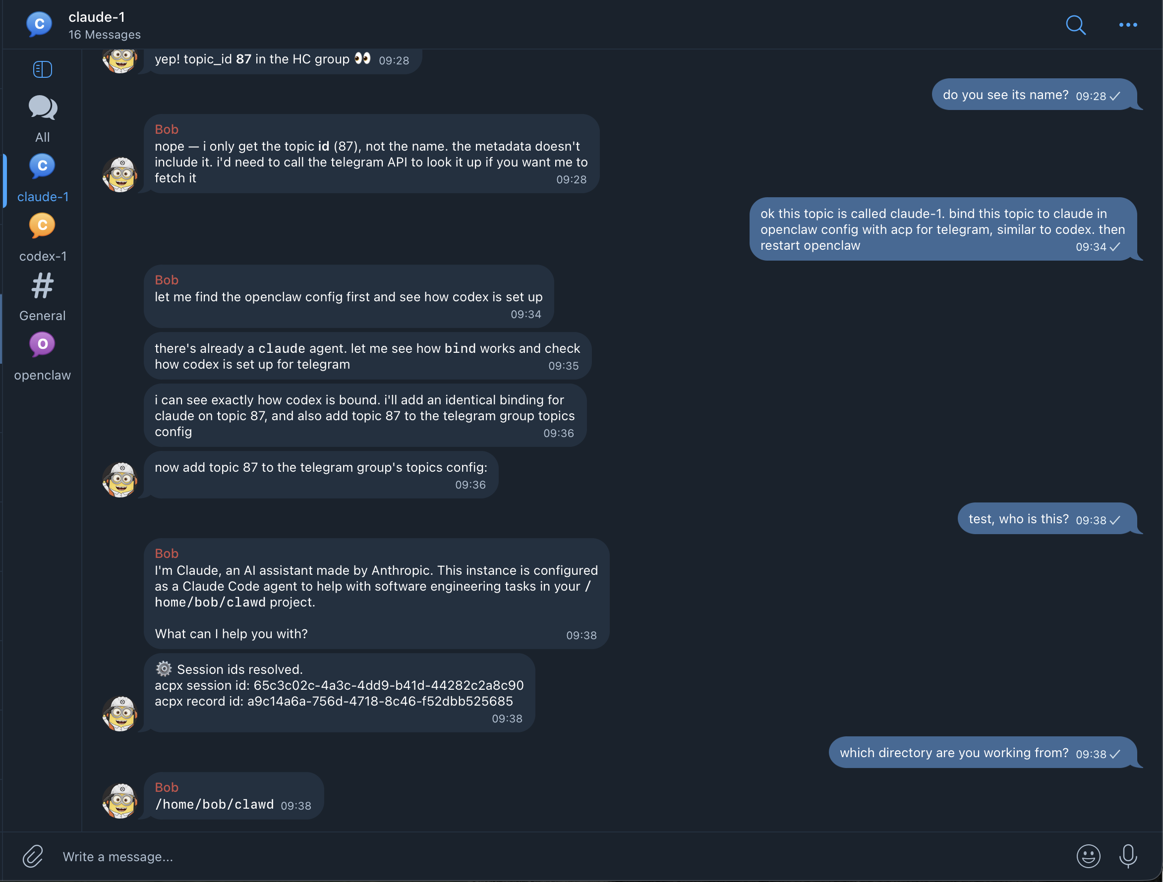
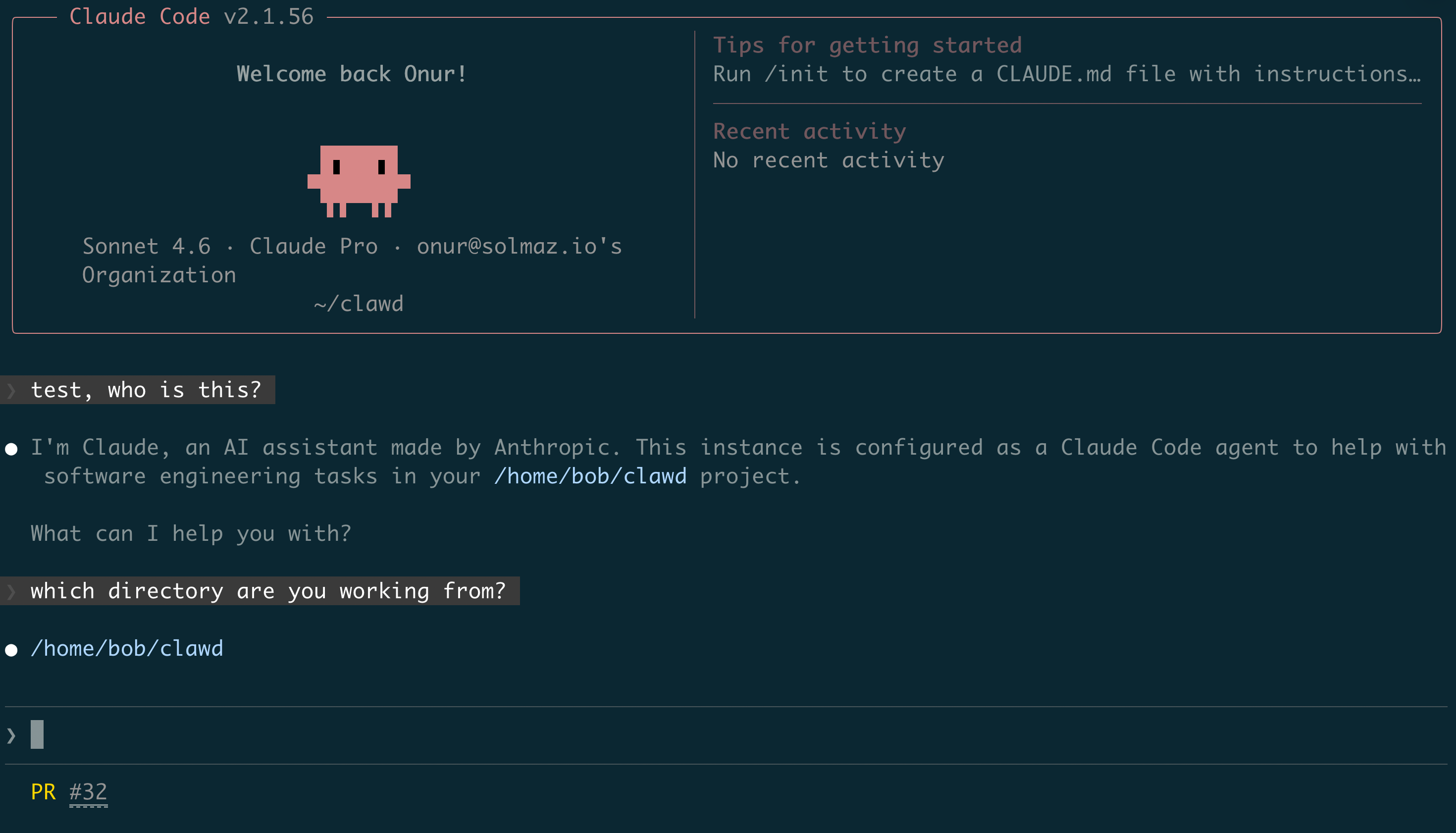

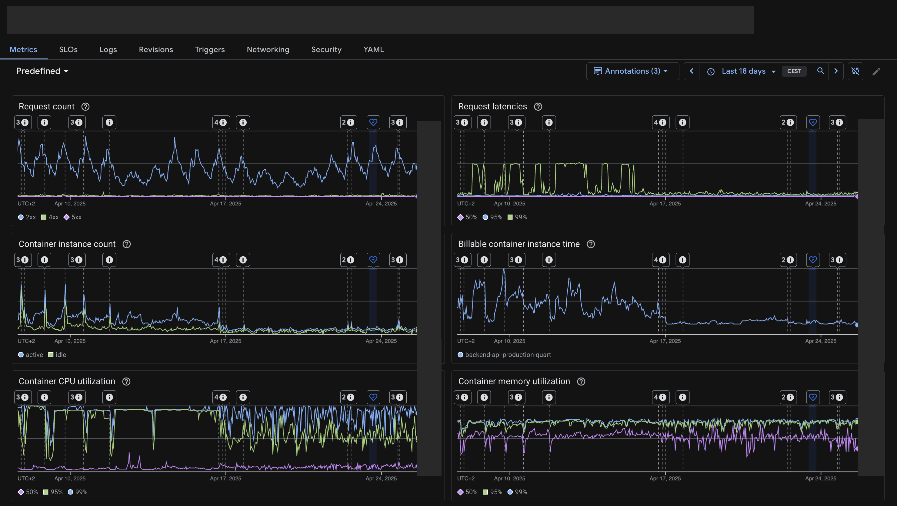
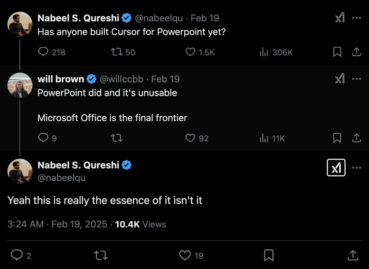


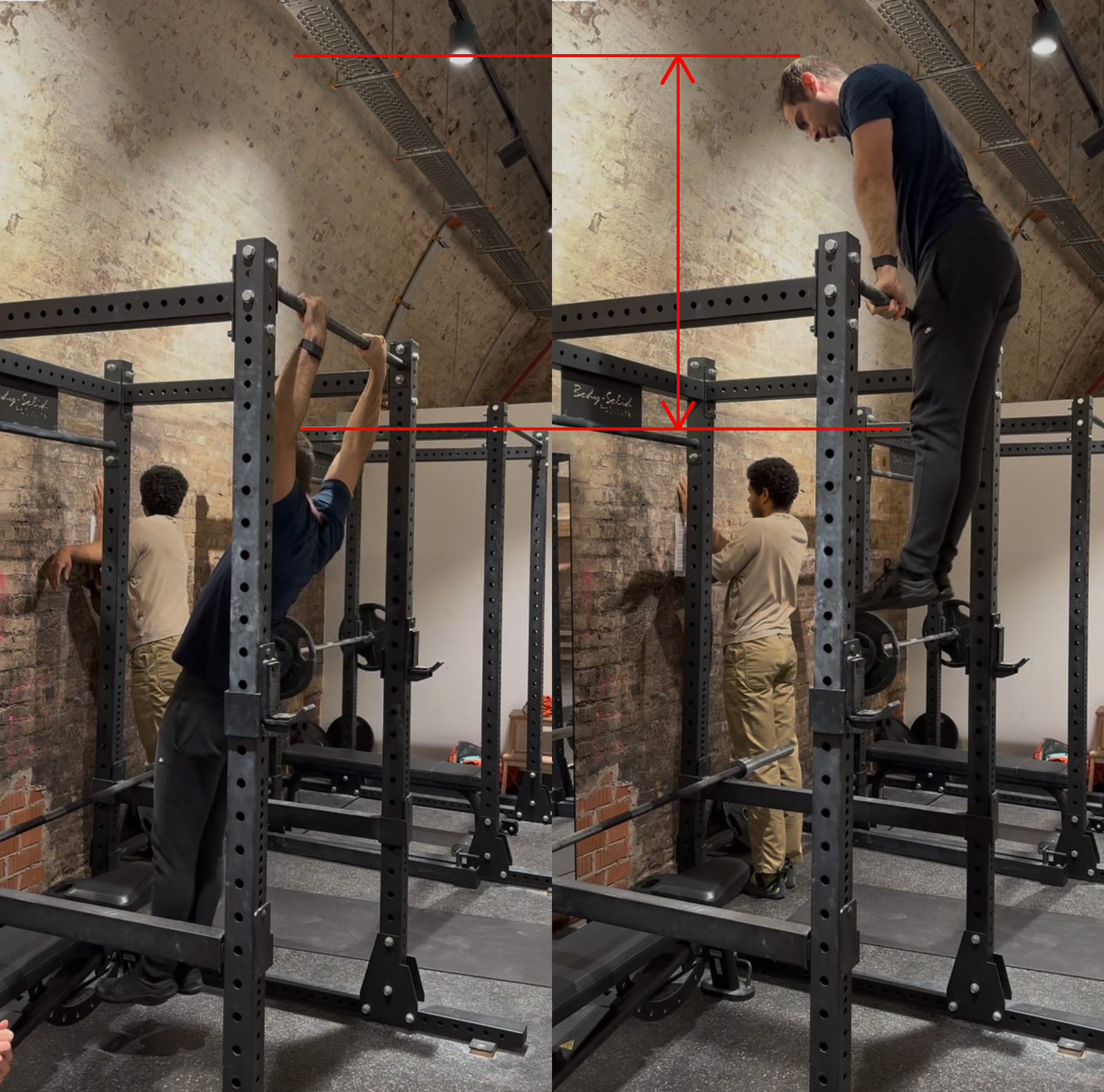


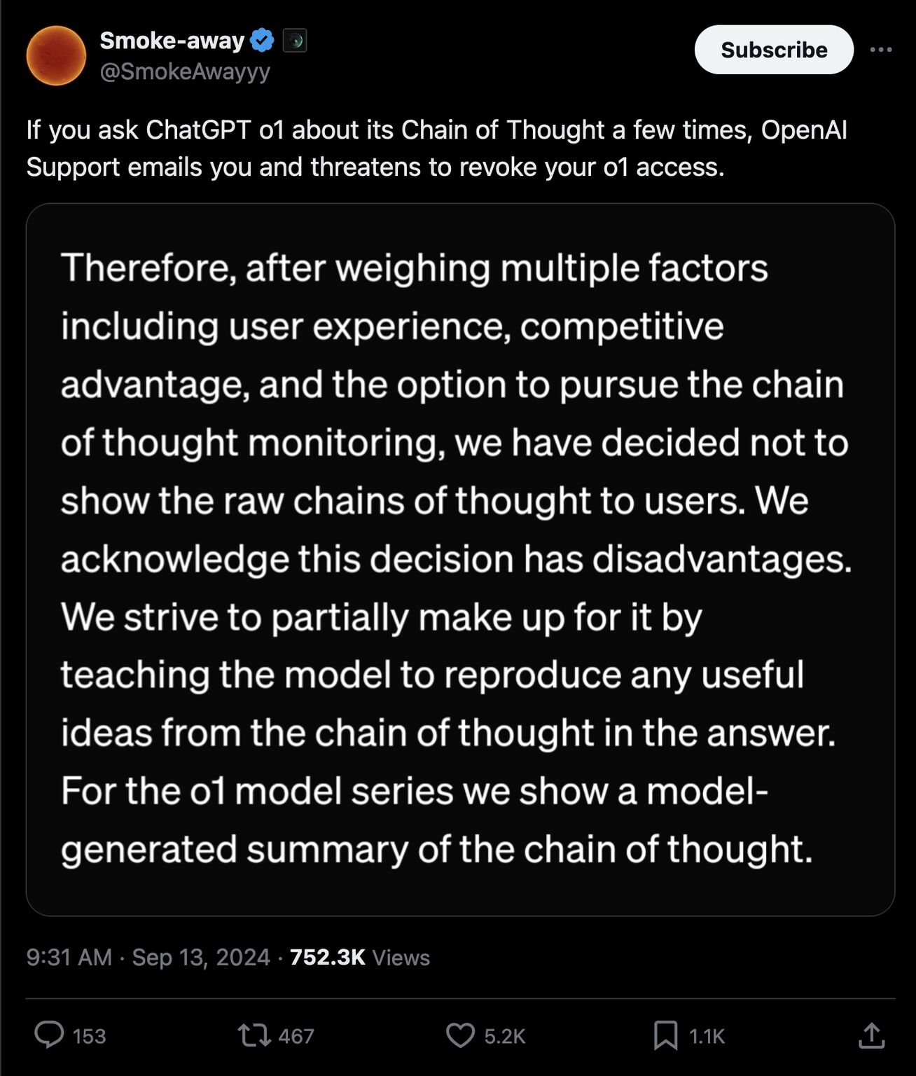
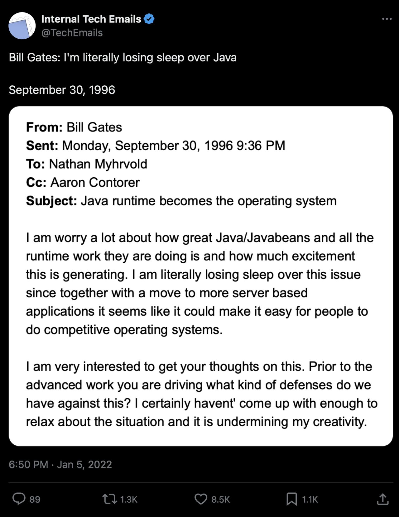
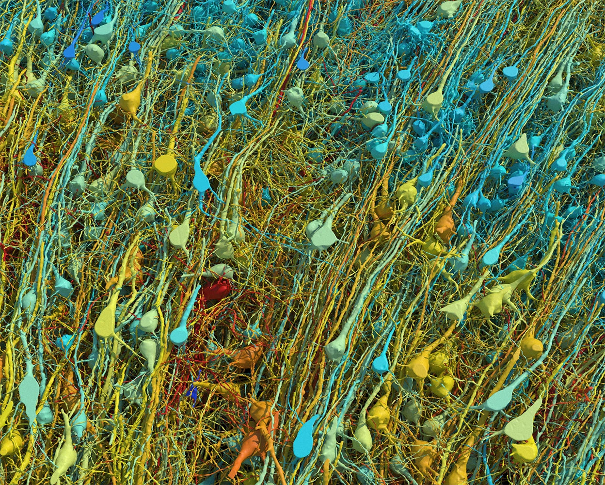


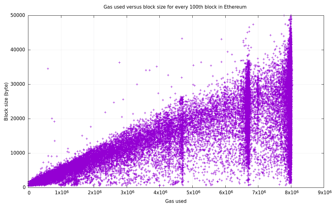


 Number of nodes $N$ versus $P R_0/c_f$, on a log scale. The
straight lines were
solved for numerically, and corresponding approximations were overlaid with
markers, except for $\alpha=1$ and $2$.
Number of nodes $N$ versus $P R_0/c_f$, on a log scale. The
straight lines were
solved for numerically, and corresponding approximations were overlaid with
markers, except for $\alpha=1$ and $2$. Bitcoin inflation rate versus block height.
 Bitcoin supply versus block height.
 An example supply versus price graph. The area below the curve is equal to the amount of ETH $E$ that must be spent to increase the supply from $S_0$ to $S_1$, or that is going to be received when $S_1-S_0$ tokens are unbonded.
 $S_0$ versus $E^{\text{suff}}_2$ for $E_1 = 100$.
 Logarithmic plot of $S_0$ versus $E^{\text{suff}}_2$ for changing values of $E_1$.
 $S_0$ versus $T^{\text{suff}}_2$ for $E_1 = 100$.
 Commutative diagram for the pull-back and push-forward relationships of the Green-Lagrange and
Almansi strain tensors.
Commutative diagram for the pull-back and push-forward relationships of the Green-Lagrange and
Almansi strain tensors. Commutative diagram of the linearized solution procedure. Each
iteration brings the current iterate $\bar{\Bvarphi}$ closer to the optimum
value $\Bvarphi^\ast$.
Commutative diagram of the linearized solution procedure. Each
iteration brings the current iterate $\bar{\Bvarphi}$ closer to the optimum
value $\Bvarphi^\ast$. Mappings between line elements belonging to the tangent spaces of
the linearization.
Mappings between line elements belonging to the tangent spaces of
the linearization.


 Commutative diagrams involving
the linear mappings $\BP,\BQ,\BR,\BS$ and
their dual $\BP^\ast,\BQ^\ast,\BR^\ast,\BS^\ast$
based on the metrics $\BG$ and $\Bg$
of $\CV$ and $\CW$.
Commutative diagrams involving
the linear mappings $\BP,\BQ,\BR,\BS$ and
their dual $\BP^\ast,\BQ^\ast,\BR^\ast,\BS^\ast$
based on the metrics $\BG$ and $\Bg$
of $\CV$ and $\CW$.
 A body $\CB$ embedded in $\IR^2$ with curvilinear coordinates.
Every point $\CP$ at $\BX$ has an associated two-dimensional vector space,
called $\CB$’s tangent space at $\BX$, denoted $\tang_\BX\CB$. The basis
$\Be_i$ corresponding to coordinates $\theta_i$ are not necessarily
orthogonal and can admit corresponding duals $\Be^i$, due to
curvilinearity.
The coordinates appear to be affine at the point’s immediate vicinity,
and thus in the tangent space.
A body $\CB$ embedded in $\IR^2$ with curvilinear coordinates.
Every point $\CP$ at $\BX$ has an associated two-dimensional vector space,
called $\CB$’s tangent space at $\BX$, denoted $\tang_\BX\CB$. The basis
$\Be_i$ corresponding to coordinates $\theta_i$ are not necessarily
orthogonal and can admit corresponding duals $\Be^i$, due to
curvilinearity.
The coordinates appear to be affine at the point’s immediate vicinity,
and thus in the tangent space.