Entries for 2018
-

The Anatomy of a Block Stuffing Attack
Block stuffing is a type of attack in blockchains where an attacker submits transactions that deliberately fill up the block’s gas limit and stall other transactions. To ensure inclusion of their transactions by miners, the attacker can choose to pay higher transaction fees. By controlling the amount of gas spent by their transactions, the attacker can influence the number of transactions that get to be included in the block.
To control the amount of gas spent by the transaction, the attacker utilizes a special contract. There is a function in the contract which takes as input the amount of gas that the attacker wants to burn. The function runs meaningless instructions in a loop, and either returns or throws an error when the desired amount is burned.
For example let’s say that the average gas price has been 5 Gwei in the last 10 blocks. In order to exert influence over the next block, the attacker needs to submit transactions with gas prices higher than that, say 100 Gwei. The higher the gas price, the higher the chance of inclusion by miners. The attacker can choose to divide the task of using 8,000,000 gas—current gas limit for blocks—into as many transactions as they want. This could be 80 transactions with 100,000 gas expenditure, or 4 transactions with 2,000,000 gas expenditure.
Deciding on how to divide the task is a matter of maximizing the chance of inclusion, and depends on the factors outline below.
Miners’ strategy for selecting transactions
Miners want to maximize their profit by including transactions with highest fees. In the current PoW implementation of Ethereum, mining the block takes significantly more time than executing the transactions. So let’s assume all transactions in the pool are trivially executed as soon as they arrive and miners know the amount of gas each one uses.
For miners, maximizing profit is an optimum packing problem. Miners want to choose a subset of the transaction pool that gives them maximum profit per block. Since there are at least tens of thousands of transactions in the pool at any given time, the problem can’t be solved by brute-forcing every combination. Miners use algorithms that test a feasible number of combinations and select the one giving the highest reward.
A block stuffer’s main goal is to target the selection process by crafting a set of transactions that has the highest chance of being picked up by miners in a way that will deplete blocks’ gas limits. They can’t devise a 100% guaranteed strategy since each miner can use a different algorithm, but they can find a sweet spot by testing out the whole network.
(In a PoS system, our assumptions would be wrong since executing transactions is not trivial compared to validating blocks. Validators would need to develop more complex strategies depending on the PoS implementation.)
The transactions the attacker wants to stall:
It could be so that the attacker wants to stall transactions with a specific contract. If the function calls to that contract use a distinctively high amount of gas, say between 300,000 and 500,000, then the attacker has to stuff the block in a way that targets that range.
For example, the attacker can periodically submit transactions with very high prices where
If the attacker is targeting transactions within a range of , they can choose the first transactions to deplete gas in short steps, and submit to deplete the remaining gas with a relatively higher price. Note that the revenue from including a single transaction is
As gas usage decreases, the probability of being picked up by miners decreases, so prices should increase to compensate.
Example: Fomo3D
Fomo3D is a gambling game where players buy keys from a contract and their money goes into a pot. At the beginning of each round, a time counter is initiated which starts counting back from 24 hours. Each bought key adds 30 seconds to the counter. When the counter hits 0, the last player to have bought a key wins the majority of the pot and the rest is distributed to others. The way the pot is distributed depends on the team that the winner belongs to.
Key price increases with increasing key supply, which makes it harder and harder to buy a key and ensures the round will end after some point. In time, the stakes increase and the counter reduces to a minimum, like 2 minutes. At this point, the players pay both high gas and key prices to be “it” and win the game. Players program bots to buy keys for them, and winning becomes a matter of coding the right strategy. As you can understand from the subject, the first round was won through a block stuffing attack.
On August 22 2018, the address 0xa16…f85 won 10,469 ETH from the first round by following the strategy I outlined above. The winner managed to be the last buyer in block 6191896 and managed to stall transactions with Fomo3D until block 6191909 for 175 seconds, ending the round. Some details:
-
Fomo3D Long contract address: 0xA62…Da1
-
Last transaction by the winner before the attack starts: 0x7a0…349
-
Transaction ending the round and firing the
onBuyAndDistributeevent which distributes the pot: 0xa14…012 -
Transaction where winner withdraws the prize: 0xe08…508
-
Contract used for block stuffing: 0x18e…801
-
Other addresses possibly belonging to the winner: 0x3c3…f27, 0xc6a…3e2, 0x81e…0ac, 0xc96…590, 0xd27…642, 0x18d…a9a, 0x87c…4ef, 0x9da…0cf, 0x7dd…c4c, 0xb1d…aef, 0x1a6…d56, 0xf6e…059, 0x1dd…a69, 0x061…63b, 0x00c…776, 0xa94…eb8, 0xf03…1f2
-
Other contracts possibly deployed by the winner for testing prior to the attack: 0xaf1…eae, 0x0c0…5ad, 0x88e…d04, 0x4f4…6f8, 0x487…4e5
The user addresses above were scraped from the Ethereum transaction graph as being linked to a primary account which supplied them with funds. The contract addresses were scraped from 0-valued transactions sent from user addresses. These have a distance of 1, there may be other addresses involved with greater distances.
Below are details of the last 4 blocks preceding the end of the round. The rows highlighted with yellow are transactions submitted by the attacker. The crossed out rows are failed transactions. All transactions by the attacker were submitted with a 501 Gwei gas price, and stuffing a single block costed around 4 ETH. The calls to buy keys generally spend around 300,000~500,000 gas, depending on which function was called. Below, you see the successfully stuffed block 6191906.
Block 6191906 Idx From To Hash ETH sent Gas Price
[Gwei]Gas Limit Gas Used ETH spent
on gas0 0xF03…1f2 0x18e…801 0xb97…8e4 0 501.0 4,200,000 4,200,000 2.1042 1 0x87C…4eF 0x18e…801 0x96f…1b0 0 501.0 3,600,000 3,600,000 1.8036 2 0xf6E…059 0x18e…801 0x897…2b3 0 501.0 200,000 200,000 0.1002 Sum 0 1503.01 8,000,000 8,000,000 4.0080 Block 6191907 was a close call for the winner, because their transactions picked up for the block did not amount up to 8,000,000 and the other transaction was a call to Fomo3D by an opponent to buy keys. Note that it has a gas price of 5559 Gwei, which means either the bot or person who submitted the transaction was presumably aware of the attack. The transaction failed due to low gas limit, presumably due to a miscalculation by the bot or the person.
Block 6191907 Idx From To Hash ETH sent Gas Price
[Gwei]Gas Limit Gas Used ETH spent
on gas0 0x32A…370 0xA62…Da1 0x5e7…be1 0.0056 5559.7 379,000 379,000 2.1071 1 0xC6A…3E2 0x18e…801 0xb8b…40c 0 501.0 3,900,000 3,900,000 1.9539 2 0xD27…642 0x18e…801 0xbcf…c62 0 501.0 3,300,000 3,300,000 1.6533 3 0x00c…776 0x18e…801 0xf30…337 0 501.0 400,000 400,000 0.2004 Sum 0.0056 7062.71 7,979,000 7,979,000 5.9147 Transactions in block 6191908 belonged to the attacker except for one irrelevant transfer. This block is also considered successfully stuffed, since the 7,970,000 gas usage by the attacker leaves no space for a call to buy keys.
Block 6191908 Idx From To Hash ETH sent Gas Price
[Gwei]Gas Limit Gas Used ETH spent
on gas0 0xD27…642 0x18e…801 0x74a…9b1 0 501.0 3,300,000 3,300,000 1.6533 1 0x7Dd…c4c 0x18e…801 0x48c…222 0 501.0 2,700,000 2,700,000 1.3527 2 0x3C3…f27 0x18e…801 0x01b…4aa 0 501.0 1,800,000 1,800,000 0.9018 3 0xa94…eb8 0x18e…801 0x776…d43 0 501.0 170,000 170,000 0.0851 4 0xbFd…1b4 0x663…d31 0x3a6…ba1 0.05 100.0 21,000 21,000 0.0021 Sum 0.05 2104.01 7,991,000 7,991,000 3.9950 By block 6191909, the counter has struck zero—more like current UTC time surpassed the round end variable stored in the contract—and any call to Fomo3D would be the one to end the round and distribute the pot. And the first transaction in the block is—wait for it—a call to Fomo3D to buy keys by the opponent whose transaction failed a few blocks earlier, submitted with 5562 Gwei. So the guy basically paid 1.7 ETH to declare the attacker the winner!
Block 6191909 Idx From To Hash ETH sent Gas Price
[Gwei]Gas Limit Gas Used ETH spent
on gas0 0x32A…370 0xA62…Da1 0xa14…012 0.0056 5562.2 379,000 304,750 1.6950 1 0xC96…590 0x18e…801 0xf47…9ca 0 501.0 2,200,000 37,633 0.0188 2 0xb1D…aEF 0x18e…801 0xe4c…edb 0 501.0 1,400,000 37,633 0.0188 3 0x18D…A9A 0x18e…801 0xf3a…995 0 501.0 800,000 37,633 0.0188 … … … … … … … … … Another thing to note is that the attacker probably crafted the spender contract to stop the attack when the round has ended, presumably to cut costs. So the 37,633 gas used by the contract are probably to call the Fomo3D contract to check round status. All these point out to the fact that the attacker is an experienced programmer who knows their way around Ethereum.
Here, you can see the details of the 100 blocks preceding the end of the round, with the additional information of ABI calls and events fired in transactions.
Since the end of the first round, 2 more rounds ended with attacks similar to this one. I didn’t analyze all of them because it’s too much for this post, but here are some details if you want to do it yourselves.
Round Address winning the pot Winner’s last tx before the end of the round Block containing that tx Tx ending the round Block containing that tx Tx where winner withdraws prize Amount won [ETH] Contract used for block stuffing 1 0xa169df5ed3363cfc4c92ac96c6c5f2a42fccbf85 0x7a06d9f11e650fbb2061b320442e26b4a704e1277547e943d73e5b67eb49c349 6191896 0xa143a1ee36e1065c3388440ef7e7b38ed41925ca4799c8a4d429fa3ee1966012 6191909 0xe08a519c03cb0aed0e04b33104112d65fa1d3a48cd3aeab65f047b2abce9d508 10,469 0x18e1b664c6a2e88b93c1b71f61cbf76a726b7801 2 0x18a0451ea56fd4ff58f59837e9ec30f346ffdca5 0x0437885fa741f93acfdcda9f5a2e673bb16d26dd22dfc4890775efb8a94fb583 6391537 0x87bf726bc60540c6b91cc013b48024a5b8c1431e0847aadecf0e92c56f8f46fd 6391548 0x4da4052d2baffdc9c0b82d628b87d2c76368914e33799032c6966ee8a3c216a0 3,264 0x705203fc06027379681AEf47c08fe679bc4A58e1 3 0xaf492045962428a15903625B1a9ECF438890eF92 0x88452b56e9aa58b70321ee8d5c9ac762a62509c98d9a29a4d64d6caae49ae757 6507761 0xe6a5a10ec91d12e3fec7e17b0dfbb983e00ffe93d61225735af2e1a8eabde003 6507774 0xd7e70fdf58aca40139246a324e871c84d988cfaff673c9e5f384315c91afa5e4 376 0xdcC655B2665A675B90ED2527354C18596276B0de A thing to note in the following rounds is that participation in the game and amount of pot gradually decreased, presumably owing to the fact that the way of beating the game has been systematized. Although anyone can attempt such an attack, knowing how it will be won takes the “fun” factor out of it.
Credit: Although I’ve found previous instances of the term “block stuffing” online, Nic Carter is the first one to use it in this context.
-
-
Mathematics of Bonding Curves
A bonding curve is a financial instrument proposed by Simon de la Rouviere in his Medium articles. ETH is bonded in a smart contract to mint tokens, and unbonded to burn them. Every bonding and unbonding changes the price of the token according to a predefined formula. The “curves” represent the relationship between the price of a single token and the token supply. The result is an ETH-backed token that rewards early adopters.
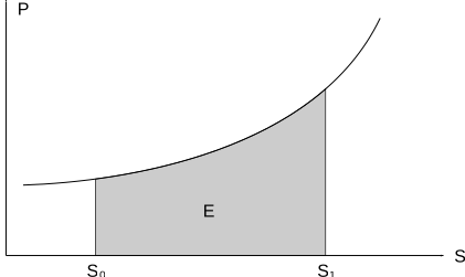 An example supply versus price graph. The area below the curve is equal to the amount of ETH that must be spent to increase the supply from to , or that is going to be received when tokens are unbonded.
Inside a transaction, the price paid/received per token is not constant and depends on the amount that is bonded or unbonded. This complicates the calculations.
Let’s say for an initial supply of , we want to bond tokens which are added to the new supply . The ETH that must be spent for this bonding is defined as
which is illustrated in the figure above. If one wanted to unbond tokens, the upper limit for the integral would be and the lower , with E corresponding to the amount of ETH received for the unbonding.
Linear Curves
A linear relationship for the bonding curves are defined as
where is the initial price of the token and is the price increment per token.
Bonding Tokens
Let us have ETH which we want to bond tokens with. Substituting into the integral above with the limits , we obtain in terms of the tokens that we want to bond:
where is the supply before the bonding. Solving this for , we obtain the tokens received in a bonding as a function of the supply and ETH spent:
Unbonding Tokens
Let us have T tokens which we want to unbond for ETH. Unbonding tokens decreases the supply from to , which we apply as limits for the above integral and obtain:
Breaking Even in PoWH3D
PoWH3D is one of the applications of bonding curves with a twist: 1/10th of every transaction is distributed among token holders as dividends. When you bond tokens with ETH, you receive worth of tokens and is distributed to everybody else in proportion to the amount they hold.
This means you are at a loss when you bond P3D (the token used by PoWH3D). If you were to unbond immediately, you would only receive 81% of your money. Given the situation, one wonders when exactly one can break even with their investment. The activity in PoWH3D isn’t deterministic; nonetheless we can deduce sufficient but not necessary conditions for breaking even in PoWH3D.
Sufficient Bonding
Let us spend ETH to bond tokens at supply . The following calculations are done with the assumption that the tokens received
are small enough to be neglected, that is and . In other words, this only holds for non-whale bondings.
Then let others spend ETH to bond tokens and raise the supply to . The objective is to find an large enough to earn us dividends and make us break even when we unbond our tokens at . We have
Our new share of the P3D pool is and the dividends we earn from the bonding is equal to
Then the condition for breaking even is
This inequality has a lengthy analytic solution which is impractical to typeset. The definition should be enough:
}\left\{\frac{9}{10} E(S_2, T_1) + \frac{1}{10}\frac{T_1}{S_2}E_2 = E_1\right\}and
can be obtained from the source of this page in JavaScript from the function
sufficient_bonding. The function involves many power and square operations and may yield inexact results for too high values of or too small values off , due to insufficient precision of the underlying math functions. For this reason, the calculator is disabled for sensitive input.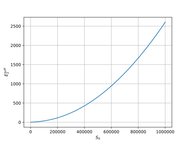 versus for .
The relationship between the initial supply and sufficient bonding is roughly quadratic, as seen from the graph above. This means that the difficulty of breaking even increases quadratically as more people bond into P3D. As interest in PoWH3D saturates, dividends received from the supply increase decreases quadratically.
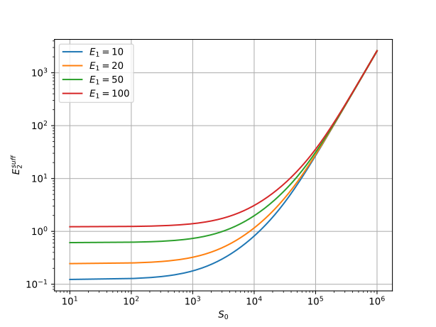 Logarithmic plot of versus for changing values of .
The relationship is not exactly quadratic, as seen from the graph above. The function is sensitive to for small values of .
Sufficient Unbonding
Let us spend ETH to bond tokens at supply and receive tokens.
Then let others unbond P3D to lower the supply to . The objective is to find a large enough to earn us dividends and make us break even when we unbond our tokens at . We have
Our new share of the P3D pool is and the dividends we earn from the bonding is equal to
Then the condition for breaking even is
Similar to the previous section, we have
}\left\{\frac{9}{10} E(S_2, T_1) + \frac{1}{10}\frac{T_1}{S_2} E(S_2, T_2) = E_1\right\}and
can be obtained from the function
sufficient_unbonding.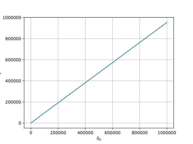 versus for .
The relationship between and is linear and insensitive to . Regardless of the ETH you invest, the amount of tokens that need to be unbonded to guarantee your break-even is roughly the same, depending on your entry point.
Calculator
Below is a calculator you can input and to calculate and .
For the default values above, we read this as:
For 100 ETH worth of P3D bonded at 3,500,000 supply, either a bonding of ~31715 ETH or an unbonding of ~3336785 P3D made by other people is sufficient to break even.
In order to follow these statistics, you can follow this site.
Conclusion
Bonding curve calculations can get complicated because the price paid per token depends on the amount of intended bonding/unbonding. With this work, I aimed to clarify the logic behind PoWH3D. Use the formulation and calculator at your own risk.
The above conditions are only sufficient and not necessary to break even. As PoWH3D becomes more popular, it gets quadratically more difficult to break even from a supply increase. PoWH3D itself doesn’t generate any value or promise long-term returns for its holders. However every bond, unbond and transfer deliver dividends. According to its creators, P3D is intended to become the base token for a number of games that will be built upon PoWH3D, like FOMO3D.
-
Lumped L2 Projection
When utilizing Galerkin-type solutions for IBVPs, we often have to compute integrals using numerical methods such as Gauss quadrature. In such a solution, we solve for the values of a function at mesh nodes, whereas the integration takes place at the quadrature points. Depending on the case, we may need to compute the values of a function at mesh nodes, given their values at quadrature points, e.g. stress recovery for mechanical problems.
There are many ways of achieving this, such as superconvergent patch recovery. In this post, I wanted to document a widely used solution which is easy to implement, and which is used in research oriented codebases such as FEAP.
L2 Projection
Given a function , its projection into a finite element space is defined through the following optimization problem:
Find such that
There is a unique solution to the problem since is convex. Taking its variation, we have $$
for all . Thus we have the following variational formulation
Find such that
for all .
Here,
are our bilinear and linear forms respectively. Substituting FE discretizations and , we have
for , where the FE matrix and vector are defined as
Thus L2 projection requires the solution of a linear system
which depending on the algorithm used, can have a complexity of at least and at most .
Lumped L2 Projection
The L2 projection requires the solution of a system which can be computationally expensive. It is possible to convert the matrix—called the mass matrix in literature—to a diagonal form through a procedure called lumping.
The operator for row summation is defined as
For the mass matrix, we have
since . Substituting the lumped mass matrix allows us to decouple the linear system of equations in (5) and instead write
for . The lumped L2 projection is then as simple as
This results in a very efficient algorithm with complexity.
Conclusion
Lumped L2 projection is a faster working approximation to L2 projection that is easy to implement for quick results. You can use it when developing a solution for an IBVP, and don’t want to wait too long when debugging, while not forgetting that it introduces some error.
-
Disadvantages of Engineering Notation in Finite Elements
Suppose we have the following stiffness matrix of linear elasticity:
where are the gradients of the shape functions and is the linear elasticity tensor (you see the contraction of their components in the equation).
Despite being of the most explicit form, these types of indicial expressions are avoided in most texts on finite elements. There are two reasons for this:
- Engineers are not taught the Einstein summation convention.
- The presence of indices result in a seemingly cluttered expression.
They avoid the indicial expression by reshaping it into matrix multiplications. In engineering notation, the left- and right-hand sides are reshaped as
which allows us to write
The matrices and are set on with tildes in order to differentiate them from the boldface symbols used in the previous sections. Here,
- is a matrix containing the unique components of the elasticity tensor , according to the Voigt notation. In this reshaping, only the minor symmetries are taken into account. If the dimension of the vectorial problem is , then is of the size . For example, if the problem is 3 dimensional, is of the size :
- is a matrix whose components are adjusted so that (2) is equivalent to (1). It has the components of for where is the number of basis functions. Since is adjusted to account for the reshaping of , it has many zero components. A 3d example:
Although (3) looks nice on paper, it is much less optimal for implementation. Implementing it requires the implementation of (5), which adds another layer of complexity to the algorithm. The same cannot be said for (4), because using Voigt notation might be more efficient in inelastic problems. In the most complex problems, the most efficient method is to implement (1) in conjunction with Voigt notation.
To prove the inefficiency of (3) we can readily compare it with (1) in terms of required number of iterations. Indices in (1) have the following ranges:
so iterations are required. Indices in (2) have the following ranges:
so
iterations are required. So engineering notation requires times more equations than index notation. For , engineering notation is times slower and for it is times slower. For example, calculation of a stiffness matrix for and requires iterations for engineering notation, whereas it only requires iterations for index notation.
Although (3) seems less cluttered, what actually happens is that one trades off complexity in one expression for a much increased complexity in another one, in this case (5). And to make it worse, it results in a slower algorithm.
The only obstacle to the widespread adoption of index notation seems to be its lack in undergraduate engineering curricula. If engineers were taught the index notation and summation convention as well as the formal notation, such expressions would not be as confusing at first sight. A good place would be in elementary calculus and physics courses, where one heavily uses vector calculus.
-
Variational Formulation of Elasticity
There are many books that give an outline of hyperelasticity, but there are few that try to help the reader implement solutions, and even fewer that manage to do it in a concise manner. Peter Wriggers’ Nonlinear Finite Element Methods is a great reference for those who like to roll up their sleeves and get lost in theory. It helped me understand a lot about how solutions to hyperelastic and inelastic problems are implemented.
One thing did not quite fit my taste though—it was very formal in the way that it didn’t give out indicial expressions. And if it wasn’t clear up until this point, I love indicial expressions, because they pack enough information to implement a solution in a single line. Almost all books skip these because they seem cluttered and the professors who wrote them think they’re trivial to derive. In fact, they are not. So below, I’ll try to derive indicial expressions for the update equations of hyperelasticity.
In the case of a hyperelastic material, there exists a strain energy function
which describes the elastic energy stored in the solid, i.e. energy density per unit mass of the reference configuration. The total energy stored in is described by the the stored energy functional
The loads acting on the body also form a potential:
where and are the prescribed body forces per unit mass and surface tractions respectively, where with Cauchy’s stress theorem.
The potential energy of for deformation is defined as
Thus the variational formulation reads
Find such that the functional
is minimized for on .
The solution is one that minimizes the potential energy:
A stationary point for means that its first variation vanishes: .
Using and ,
The symmetric part of the term on the right hand side of the contraction is equal to the variation of the Green-Lagrange strain tensor:
Substituting, we obtain the semilinear form in terms of the second Piola-Kirchhoff stress tensor:
We can write a Eulerian version of this form by pushing-forward the stresses and strains. The Almansi strain is the pull-back of the Green-Lagrange strain and vice versa:
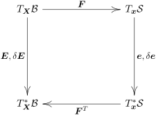 Commutative diagram for the pull-back and push-forward relationships of the Green-Lagrange and
Almansi strain tensors.
Commutative diagram for the pull-back and push-forward relationships of the Green-Lagrange and
Almansi strain tensors.
Thus we can deduce the variation of the Almansi strain
where we have used the identity
The second Piola-Kirchhoff stress is the pull-back of the Kirchhoff stress :
Then it is evident that
We can thus write the Eulerian version of (10):
Introducing the Cauchy stresses , we can also transport the integrals to the current configuration
Here, we substituted the following differential identities:
for the body forces, and
for the surface tractions, where we used the Piola identity.
Linearization of the Variational Formulation
We linearize :
Then we have the variational setting
where
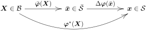 Commutative diagram of the linearized solution procedure. Each
iteration brings the current iterate closer to the optimum
value .
Commutative diagram of the linearized solution procedure. Each
iteration brings the current iterate closer to the optimum
value .
 Mappings between line elements belonging to the tangent spaces of
the linearization.
Mappings between line elements belonging to the tangent spaces of
the linearization.
The variation is calculated as
Consecutive variations of the Green-Lagrange strain tensor is calculated as
The term on the left is calculated as
where we substitute the Lagrangian elasticity tensor
and is calculated in the same manner as :
Then the variational forms of the linearized setting are
where the bars denote evaluation of dependent variables.
Eulerian Version of the Linearization
We also have the following relationship between the Lagrangian and Eulerian elasticity tensors
Substituting Eulerian expansions, we obtain the following identity:
Thus we have
With these results at hand, we can write the Eulerian version of our variational formulation:
If we introduce the Cauchy stress tensor and corresponding elasticity tensor , our variational formulation can be expressed completely in terms of Eulerian quantities:
We have the following relationships of the differential forms:
where and .
Discretization of the Lagrangian Form
We use the following FE discretization:
where is the number of element nodes and is the number of spatial dimensions.
We use the same discretization for and . Then the linear system at hand becomes
for and where the and are calculated from the variational forms as
For detailed derivation, see the post Vectorial Finite Elements.
For discretized gradients, we have the following relationship
where . For the first term in , we can get rid of the symmetries:
and for the second term, we have
where are the components of the Eulerian metric tensor.
For the first term in , we have
Remaining terms can be calculated in a straightforward manner. We then have for and :
The lowercase indices in and might be confusing, but in fact
The system is solved for at each Newton iteration with the following update equation:
Discretization of the Eulerian Form
Discretization of the Eulerian formulation parallels that of Lagrangian.
Here, denote the spatial gradients of the shape functions. One way of calculating is , similar to (13).
The update equation (44) holds for the Eulerian version.
Conclusion
The equations above in boxes contain all the information needed to implement the nonlinear solution scheme of hyperelasticity.
-
Discontinuous Divergence Theorem
In lecture notes related to the Discontinuous Galerkin method, there is mention of a magic formula which AFAIK first appeared on a paper1 by Douglas Arnold (at least in this context).
It has been proven and all, but it’s still called magic because its reasoning is not apparent at first glance. The magic formula is actually a superset of the divergence theorem, generalized to discontinuous fields. But to make that generalization, we need to abandon the standard formulation which starts by creating a triangular mesh, and consider arbitrary partitionings of a domain.
A domain is partitioned into parts , as follows:
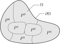
We call the set of parts a partition of .
Broken Hilbert Spaces
We allow the vector field to be discontinuous at boundaries and continuous in , . To this end, we define the broken Hilbert space over partition
It can be seen that .
Part Boundaries
Topologically, a part may share boundary with , like . In that case, the boundary of the part is divided into an interior boundary and exterior boundary:
If a part has an exterior boundary, it is said to be an external part (, , , ). If it does not have any exterior boundary, it is said to be an internal part.(, ).
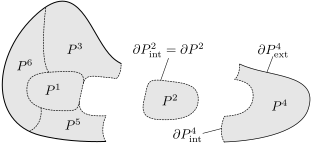
Divergence theorem over parts
For a vector field , , we can write the following integral as a sum and apply the divergence theorem afterward
We define the portion of the boundary that part shares with as the interface between and .
If and are not neighbors, we simply have .

Integrals over interior boundaries
For opposing parts and ,
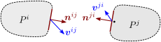
we have different values of the function and conjugate normal vectors at the interface :
Since
we can rearrange the integral over interior boundaries as
The jump operator
Integrals over the same interface can be grouped together:
Defining the jump of across
The jump of a function measures its discontinuity across interfaces. We can write
We may drop the superscripts where there is no confusion.
Interfaces and external boundaries
It is convenient to group the interfaces:
which allows us to write
It’s obvious that the union of part external boundaries equals the domain boundary:
which allows us to write
With the results obtained, we put forward a generalized version of the divergence theorem: Let be a vector field. Then we have
Verbally, the integral of the divergence of a vector field over a domain equals its integral over the domain boundary , plus the integral of its jump over part interfaces .
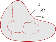
In the case of a continuous field, the jumps vanish and this reduces to the regular divergence theorem.
The Magic Formula
There are different versions of the magic formula for scalar, vector and tensor fields, and for different IBVPs. I won’t try to derive them all, but give an example: If we were substitute a linear mapping instead of , we would have the jump on the right-hand side.
We introduce the vector and tensor average operator
and tensor jump operator
We also note the boundary jump/average property which is used on the integral over
(This property is used implicitly in many places, and often causes confusion).
These definitions allow us to write the identity
which is easily proven when expanded.
The different versions of the magic formula are obtained by substituting the identities above—or their analogs—in the discontinuous divergence theorem.
-
Douglas N. Arnold. An interior penalty finite element method with discontinuous elements. SIAM J. Numer. Anal., 19(4):742–760, 1982. ↩
-