When utilizing Galerkin-type solutions for IBVPs, we often have to compute integrals using numerical methods such as Gauss quadrature. In such a solution, we solve for the values of a function at mesh nodes, whereas the integration takes place at the quadrature points. Depending on the case, we may need to compute the values of a function at mesh nodes, given their values at quadrature points, e.g. stress recovery for mechanical problems.

There are many ways of achieving this, such as superconvergent patch recovery. In this post, I wanted to document a widely used solution which is easy to implement, and which is used in research oriented codebases such as FEAP.

L2 Projection

Given a function $u \in L^2(\Omega)$, its projection into a finite element space $V_h\subset L^2(\Omega)$ is defined through the following optimization problem:

Find $u_h\in V_h$ such that

There is a unique solution to the problem since $\Pi(\cdot)$ is convex. Taking its variation, we have $$$\begin{equation} D \Pi(u_h) \cdot v_h = \langle u_h-u, v_h \rangle = 0 \tag{2}\end{equation}$$$

for all $v_h\in V_h$. Thus we have the following variational formulation

Find $u_h\in V_h$ such that

$$\begin{equation} \langle u_h,v_h\rangle = \langle u, v_h\rangle \tag{3}\end{equation}$$

for all $v_h\in V_h$.

Here,

are our bilinear and linear forms respectively. Substituting FE discretizations $u_h = \sum_{J=1}^{\nnode} u^JN^J$ and $v_h = \sum_{I=1}^{\nnode} v^IN^I$, we have

for $I=1,\dots,\nnode$, where the FE matrix and vector are defined as

Thus L2 projection requires the solution of a linear system

which depending on the algorithm used, can have a complexity of at least $O(n^2)$ and at most $O(n^3)$.

Lumped L2 Projection

The L2 projection requires the solution of a system which can be computationally expensive. It is possible to convert the matrix—called the mass matrix in literature—to a diagonal form through a procedure called lumping.

The operator for row summation is defined as

For the mass matrix, we have

since $\sum_{J=1}^{\nnode} N^J = 1$. Substituting the lumped mass matrix allows us to decouple the linear system of equations in (5) and instead write

for $I=1,\dots,\nnode$. The lumped L2 projection is then as simple as

This results in a very efficient algorithm with $O(n)$ complexity.

Conclusion

Lumped L2 projection is a faster working approximation to L2 projection that is easy to implement for quick results. You can use it when developing a solution for an IBVP, and don’t want to wait too long when debugging, while not forgetting that it introduces some error.

Suppose we have the following stiffness matrix of linear elasticity:

where $\boldsymbol{B}^I = \nabla N^I$ are the gradients of the shape functions $N^I$ and $\mathbb{C}$ is the linear elasticity tensor (you see the contraction of their components in the equation).

Despite being of the most explicit form, these types of indicial expressions are avoided in most texts on finite elements. There are two reasons for this:

• Engineers are not taught the Einstein summation convention.
• The presence of indices result in a seemingly cluttered expression.

They avoid the indicial expression by reshaping it into matrix multiplications. In engineering notation, the left- and right-hand sides are reshaped as

which allows us to write

The matrices $\tilde{\boldsymbol{B}}$ and $\tilde{\boldsymbol{C}}$ are set on with tildes in order to differentiate them from the boldface symbols used in the previous sections. Here,

• $\tilde{\boldsymbol{C}}$ is a matrix containing the unique components of the elasticity tensor $\mathbb{C}$, according to the Voigt notation. In this reshaping, only the minor symmetries are taken into account. If the dimension of the vectorial problem is $d$, then $\tilde{\boldsymbol{C}}$ is of the size $d(d+1)/2 \times d(d+1)/2$. For example, if the problem is 3 dimensional, $\tilde{\boldsymbol{C}}$ is of the size $6\times 6$:

• $\tilde{\boldsymbol{B}}$ is a $nd\times d(d+1)/2$ matrix whose components are adjusted so that (2) is equivalent to (1). It has the components of $\boldsymbol{B}^I$ for $I=1,\dots,n$ where $n$ is the number of basis functions. Since $\tilde{\boldsymbol{B}}$ is adjusted to account for the reshaping of $\mathbb{C}$, it has many zero components. A 3d example:

Although (3) looks nice on paper, it is much less optimal for implementation. Implementing it requires the implementation of (5), which adds another layer of complexity to the algorithm. The same cannot be said for (4), because using Voigt notation might be more efficient in inelastic problems. In the most complex problems, the most efficient method is to implement (1) in conjunction with Voigt notation.

To prove the inefficiency of (3) we can readily compare it with (1) in terms of required number of iterations. Indices in (1) have the following ranges:

so $n^2d^4$ iterations are required. Indices in (2) have the following ranges:

so

iterations are required. So engineering notation requires $(d+1)^2/4$ times more equations than index notation. For $d=2$, engineering notation is $2.25$ times slower and for $d=3$ it is $4$ times slower. For example, calculation of a stiffness matrix for $n=8$ and $d=3$ requires $20736$ iterations for engineering notation, whereas it only requires $5184$ iterations for index notation.

Although (3) seems less cluttered, what actually happens is that one trades off complexity in one expression for a much increased complexity in another one, in this case (5). And to make it worse, it results in a slower algorithm.

The only obstacle to the widespread adoption of index notation seems to be its lack in undergraduate engineering curricula. If engineers were taught the index notation and summation convention as well as the formal notation, such expressions would not be as confusing at first sight. A good place would be in elementary calculus and physics courses, where one heavily uses vector calculus.

There are many books that give an outline of hyperelasticity, but there are few that try to help the reader implement solutions, and even fewer that manage to do it in a concise manner. Peter Wriggers’ Nonlinear Finite Element Methods is a great reference for those who like to roll up their sleeves and get lost in theory. It helped me understand a lot about how solutions to hyperelastic and inelastic problems are implemented.

One thing did not quite fit my taste though—it was very formal in the way that it didn’t give out indicial expressions. And if it wasn’t clear up until this point, I love indicial expressions, because they pack enough information to implement a solution in a single line. Almost all books skip these because they seem cluttered and the professors who wrote them think they’re trivial to derive. In fact, they are not. So below, I’ll try to derive indicial expressions for the update equations of hyperelasticity.

In the case of a hyperelastic material, there exists a strain energy function

which describes the elastic energy stored in the solid, i.e. energy density per unit mass of the reference configuration. The total energy stored in $\CB$ is described by the the stored energy functional

The loads acting on the body also form a potential:

where $\bar{\BGamma}$ and $\bar{\BT}$ are the prescribed body forces per unit mass and surface tractions respectively, where $\BT=\BP\BN$ with Cauchy’s stress theorem.

The potential energy of $\CB$ for deformation $\Bvarphi$ is defined as

Thus the variational formulation reads

Find $\Bvarphi\in V$ such that the functional

$$\begin{equation} \Pi(\Bvarphi) = \int_{\CB} \rho_0\Psi(\BF) \dV - \int_{\CB} \rho_0\bar{\BGamma}\dtp\Bvarphi \dV - \int_{\del\CB_t} \bar{\BT}\dtp\Bvarphi \dA \tag{5}\end{equation}$$

is minimized for $\Bvarphi=\bar{\Bvarphi}$ on $\del\CB_u$.

The solution is one that minimizes the potential energy:

A stationary point for $\Pi$ means that its first variation vanishes: $\var\Pi=0$.

Using $\BP=\BF\BS$ and $\BP = \rho_0\del\Psi/\del\BF$,

The symmetric part of the term on the right hand side of the contraction is equal to the variation of the Green-Lagrange strain tensor:

Substituting, we obtain the semilinear form $G$ in terms of the second Piola-Kirchhoff stress tensor:

We can write a Eulerian version of this form by pushing-forward the stresses and strains. The Almansi strain $\Be$ is the pull-back of the Green-Lagrange strain $\BE$ and vice versa:

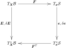Commutative diagram for the pull-back and push-forward relationships of the Green-Lagrange and Almansi strain tensors.

Thus we can deduce the variation of the Almansi strain

where we have used the identity

The second Piola-Kirchhoff stress is the pull-back of the Kirchhoff stress $\Btau$:

Then it is evident that

We can thus write the Eulerian version of (10):

Introducing the Cauchy stresses $\Bsigma=\Btau/J$, we can also transport the integrals to the current configuration

Here, we substituted the following differential identities:

for the body forces, and

for the surface tractions, where we used the Piola identity.

Linearization of the Variational Formulation

We linearize $G$:

Then we have the variational setting

where

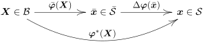Commutative diagram of the linearized solution procedure. Each iteration brings the current iterate $\bar{\Bvarphi}$ closer to the optimum value $\Bvarphi^\ast$.

Mappings between line elements belonging to the tangent spaces of the linearization.

The variation $\Var G$ is calculated as

Consecutive variations of the Green-Lagrange strain tensor is calculated as

The term on the left is calculated as

where we substitute the Lagrangian elasticity tensor

and $\Var\BE$ is calculated in the same manner as $\var\BE$:

Then the variational forms of the linearized setting are

where the bars denote evaluation $\Bvarphi=\bar{\Bvarphi}$ of dependent variables.

Eulerian Version of the Linearization

We also have the following relationship between the Lagrangian and Eulerian elasticity tensors

Substituting Eulerian expansions, we obtain the following identity:

Thus we have

With these results at hand, we can write the Eulerian version of our variational formulation:

If we introduce the Cauchy stress tensor $\Bsigma$ and corresponding elasticity tensor $\BFc^\sigma = \BFc/J$, our variational formulation can be expressed completely in terms of Eulerian quantities:

We have the following relationships of the differential forms:

where $\bar{\BF} = \nabla_X\bar{\Bvarphi}$ and $\bar{J} = \det\bar{\BF}$.

Discretization of the Lagrangian Form

We use the following FE discretization:

where $\nnode$ is the number of element nodes and $\ndim$ is the number of spatial dimensions.

We use the same discretization for $\vvphi$ and $\Vvphi$. Then the linear system at hand becomes

for $a=1,\dots,\ndim$ and $\gamma=1,\dots,\nnode$ where the $\BA$ and $\Bb$ are calculated from the variational forms as

For detailed derivation, see the post Vectorial Finite Elements.

For discretized gradients, we have the following relationship

where $\BB^\gamma:= \nabla_X N^\gamma$. For the first term in $a$, we can get rid of the symmetries:

and for the second term, we have

where $g_{ab}$ are the components of the Eulerian metric tensor.

For the first term in $b$, we have

Remaining terms can be calculated in a straightforward manner. We then have for $\BA$ and $\Bb$:

The lowercase indices in $\bar{\Bgamma}$ and $\bar{\BT}$ might be confusing, but in fact

The system is solved for $\Vvphi$ at each Newton iteration with the following update equation:

Discretization of the Eulerian Form

Discretization of the Eulerian formulation parallels that of Lagrangian.

Here, $\bar{\BB}^\gamma = \nabla_{\bar{x}} N^\gamma$ denote the spatial gradients of the shape functions. One way of calculating is $\bar{\BB}^\gamma = \bar{\BF}\invtra\BB^\gamma$, similar to (13).

The update equation (44) holds for the Eulerian version.

Conclusion

The equations above in boxes contain all the information needed to implement the nonlinear solution scheme of hyperelasticity.