There are many books that give an outline of hyperelasticity, but there are few that try to help the reader implement solutions, and even fewer that manage to do it in a concise manner. Peter Wriggers’ Nonlinear Finite Element Methods is a great reference for those who like to roll up their sleeves and get lost in theory. It helped me understand a lot about how solutions to hyperelastic and inelastic problems are implemented.

One thing did not quite fit my taste though—it was very formal in the way that it didn’t give out indicial expressions. And if it wasn’t clear up until this point, I love indicial expressions, because they pack enough information to implement a solution in a single line. Almost all books skip these because they seem cluttered and the professors who wrote them think they’re trivial to derive. In fact, they are not. So below, I’ll try to derive indicial expressions for the update equations of hyperelasticity.

In the case of a hyperelastic material, there exists a strain energy function

\begin{equation} \Psi: \BF \mapsto \Psi(\BF) \tag{1}\end{equation}

which describes the elastic energy stored in the solid, i.e. energy density per unit mass of the reference configuration. The total energy stored in $\CB$ is described by the the stored energy functional

\begin{equation} E(\Bvarphi) := \int_{\CB} \Psi(\BF)\, \dif m = \int_{\CB} \rho_0 \Psi(\BF) \dV \tag{2}\end{equation}

The loads acting on the body also form a potential:

\begin{equation} L(\Bvarphi) := \int_{\CB} \rho_0\bar{\BGamma}\dtp\Bvarphi \dV + \int_{\del\CB_t} \bar{\BT}\dtp\Bvarphi \dA \tag{3}\end{equation}

where $\bar{\BGamma}$ and $\bar{\BT}$ are the prescribed body forces per unit mass and surface tractions respectively, where $\BT=\BP\BN$ with Cauchy’s stress theorem.

The potential energy of $\CB$ for deformation $\Bvarphi$ is defined as

\begin{equation} \Pi(\Bvarphi) := E(\Bvarphi) - L(\Bvarphi) \tag{4}\end{equation}

Thus the variational formulation reads

Find $\Bvarphi\in V$ such that the functional
$\begin{equation} \Pi(\Bvarphi) = \int_{\CB} \rho_0\Psi(\BF) \dV - \int_{\CB} \rho_0\bar{\BGamma}\dtp\Bvarphi \dV - \int_{\del\CB_t} \bar{\BT}\dtp\Bvarphi \dA \tag{5}\end{equation}$
is minimized for $\Bvarphi=\bar{\Bvarphi}$ on $\del\CB_u$ .

The solution is one that minimizes the potential energy:

\begin{equation} \Bvarphi^\ast = \argmin_{\Bvarphi\in V} \Pi(\Bvarphi) \tag{6}\end{equation}

A stationary point for $\Pi$ means that its first variation vanishes: $\var\Pi=0$ .

\begin{equation} \begin{aligned} \var\Pi &= \varn{\Pi}{\Bvarphi}{\vvphi} =: G(\Bvarphi,\vvphi) \\ &= \int_{\CB} \rho_0\partd{\Psi}{\BF}: \nabla(\vvphi) \dV - \int_{\CB} \rho_0\bar{\BGamma}\dtp\vvphi \dV - \int_{\del\CB} \bar{\BT}\dtp\vvphi \dA \end{aligned} \tag{7}\end{equation}

Using $\BP=\BF\BS$ and $\BP = \rho_0\del\Psi/\del\BF$ ,

\begin{equation} \rho_0\partd{\Psi}{\BF}: \nabla(\vvphi) = \BF\BS:\nabla(\vvphi) = \BS:\BF\tra\nabla(\vvphi) \tag{8}\end{equation}

The symmetric part of the term on the right hand side of the contraction is equal to the variation of the Green-Lagrange strain tensor:

\begin{equation} \begin{aligned} \var\BE = \varn{\BE}{\Bvarphi}{\vvphi} &= \deriv{}{\eps} \frac{1}{2} [\nabla(\Bvarphi+\eps\vvphi)\tra\nabla(\Bvarphi+\eps\vvphi) - \BI]\evat_{\eps=0} \\ &= \frac{1}{2} [\nabla(\vvphi)\tra\BF + \BF\tra\nabla(\vvphi)] \end{aligned} \tag{9}\end{equation}

Substituting, we obtain the semilinear form $G$ in terms of the second Piola-Kirchhoff stress tensor:

\begin{equation} \boxed{ G(\Bvarphi,\vvphi) = \int_{\CB} \BS: \var\BE \dV - \int_{\CB} \rho_0\bar{\BGamma}\dtp\vvphi \dV - \int_{\del\CB} \bar{\BT}\dtp\vvphi \dA = 0 } \htmlId{eq:lagrangianform1}{} \tag{10}\end{equation}

We can write a Eulerian version of this form by pushing-forward the stresses and strains. The Almansi strain $\Be$ is the pull-back of the Green-Lagrange strain $\BE$ and vice versa:

\begin{equation} \Be = \push(\BE) = \BF\invtra \BE \BF\inv \eqand \BE = \pull(\Be) = \BF\tra \BE \BF \tag{11}\end{equation}

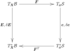
Commutative diagram for the pull-back and push-forward relationships of the Green-Lagrange and Almansi strain tensors.

Thus we can deduce the variation of the Almansi strain

\begin{equation} \begin{aligned} \var \Be = \BF\invtra \var\BE\BF\inv &= \frac{1}{2} [\nabla(\vvphi)\BF\inv+\BF\invtra \nabla(\vvphi)\tra] \\ &= \frac{1}{2} [\nabla_x(\vvphi)+ \nabla_x(\vvphi)\tra] \end{aligned} \tag{12}\end{equation}

where we have used the identity

\begin{equation} \nabla_X(\cdot)\BF\inv = \nabla_x(\cdot). \htmlId{eq:defgradidentity1}{} \tag{13}\end{equation}

The second Piola-Kirchhoff stress is the pull-back of the Kirchhoff stress $\Btau$ :

\begin{equation} \BS = \pull(\Btau) = \BF\inv\Btau\BF\invtra \tag{14}\end{equation}

Then it is evident that

\begin{equation} \BS:\var\BE = (\BF\inv\Btau\BF\invtra):(\BF\tra\var\Be\BF) = \Btau:\var\Be \tag{15}\end{equation}

We can thus write the Eulerian version of (10):

\begin{equation} \boxed{ G(\Bvarphi,\vvphi) = \int_{\CB} \Btau: \var\Be \dV - \int_{\CB} \rho_0\bar{\BGamma}\dtp\vvphi \dV - \int_{\del\CB} \bar{\BT}\dtp\vvphi \dA = 0 } \tag{16}\end{equation}

Introducing the Cauchy stresses $\Bsigma=\Btau/J$ , we can also transport the integrals to the current configuration

\begin{equation} \boxed{ G(\Bvarphi,\vvphi) = \int_{\CS} \Bsigma:\var\Be \dv - \int_{\CS} \rho\bar{\Bgamma}\dtp\vvphi \dv - \int_{\del\CS_t} \bar{\Bt}\dtp\vvphi \da = 0 } \tag{17}\end{equation}

Here, we substituted the following differential identities:

\begin{equation} \rho_0\BGamma\dV = \rho\Bgamma\dv \tag{18}\end{equation}

for the body forces, and

\begin{equation} \BT\dA = \BP\BN \dA = \Bsigma J\BF\invtra\BN \dA = \Bsigma\Bn \da = \Bt \da \tag{19}\end{equation}

for the surface tractions, where we used the Piola identity.

Linearization of the Variational Formulation

We linearize $G$ :

\begin{equation} \Lin G \evat_{\bar{\Bvarphi}} = G(\bar{\Bvarphi}, \vvphi) + \Var G \evat_{\bar{\Bvarphi}} = 0 \tag{20}\end{equation}

Then we have the variational setting

\begin{equation} a(\Vvphi,\vvphi)=b(\vvphi) \tag{21}\end{equation}

where

\begin{equation} a(\Vvphi,\vvphi) = \Var G \evat_{\bar{\Bvarphi}} \eqand b(\vvphi) = -G(\bar{\Bvarphi}, \vvphi) \tag{22}\end{equation}

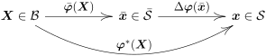
Commutative diagram of the linearized solution procedure. Each iteration brings the current iterate

\bar{\Bvarphi}

closer to the optimum value

\Bvarphi^\ast

Mappings between line elements belonging to the tangent spaces of the linearization.

The variation $\Var G$ is calculated as

\begin{equation} \Var G = \varn{G}{\Bvarphi}{\Vvphi} = \int_{\CB} [\Var\BS:\var\BE + \BS:\Var(\var\BE)] \dV \tag{23}\end{equation}

Consecutive variations of the Green-Lagrange strain tensor is calculated as

\begin{equation} \Var(\var\BE) = \varn{\var\BE}{\Bvarphi}{\Vvphi} = \frac{1}{2}[\nabla(\vvphi)\tra\nabla(\Vvphi) + \nabla(\Vvphi)\tra\nabla(\vvphi)] \tag{24}\end{equation}

The term on the left is calculated as

\begin{equation} \Var\BS = \varn{\BS}{\Bvarphi}{\Vvphi} = \partd{\BS}{\BC}:\Var\BC = 2 \partd{\BS}{\BC}:\Var\BE \tag{25}\end{equation}

where we substitute the Lagrangian elasticity tensor

\begin{equation} \BFC := 2 \partd{\BS}{\BC} = 4\rho_0 \frac{\del^2\Psi}{\del\BC\del\BC} \tag{26}\end{equation}

and $\Var\BE$ is calculated in the same manner as $\var\BE$ :

\begin{equation} \Var\BE = \frac{1}{2} [\nabla(\Vvphi)\tra\BF + \BF\tra\nabla(\Vvphi)] \tag{27}\end{equation}

Then the variational forms of the linearized setting are

\begin{equation} \boxed{ \begin{aligned} a(\Vvphi,\vvphi) &= \int_{\CB} \var\bar{\BE}:\bar{\BFC}:\Var\bar{\BE} + \bar{\BS} : [\nabla(\vvphi)\tra\nabla(\Vvphi)] \dV \\ b(\vvphi) &= - \int_{\CB} \bar{\BS}: \var\bar{\BE} \dV + \int_{\CB} \rho_0\bar{\BGamma}\dtp\vvphi \dV + \int_{\del\CB} \bar{\BT}\dtp\vvphi \dA \end{aligned} } \tag{28}\end{equation}

where the bars denote evaluation $\Bvarphi=\bar{\Bvarphi}$ of dependent variables.

Eulerian Version of the Linearization

We also have the following relationship between the Lagrangian and Eulerian elasticity tensors

\begin{equation} c_{abcd} = F_{aA}F_{bB}F_{cC}F_{dD} C_{ABCD} \tag{29}\end{equation}

Substituting Eulerian expansions, we obtain the following identity:

\begin{equation} \begin{aligned} \var\BE:\BFC:\Var\BE &= (\BF\tra\var\Be\BF):\BFC:(\BF\tra\Var\Be\BF) \\ &=F_{aA}\var e_{ab} F_{bB} C_{ABCD} F_{cC}\Var e_{cd}F_{dD} \\ &=\var e_{ab} c_{abcd} \Var e_{cd} \\ &= \var\Be:\BFc:\Var\Be \end{aligned} \tag{30}\end{equation}

Thus we have

\begin{equation} \begin{aligned} \BS:[\nabla(\vvphi)\tra\nabla(\Vvphi)] &= [\BF\inv\Btau\BF\invtra] :[\nabla(\vvphi)\tra\nabla(\Vvphi)] \\ &= \Btau : [(\nabla(\vvphi)\BF\inv)\tra\nabla(\Vvphi)\BF\inv] \\ &= \Btau : [\nabla_x(\vvphi)\tra\nabla_x(\Vvphi)] \\ \end{aligned} \tag{31}\end{equation}

With these results at hand, we can write the Eulerian version of our variational formulation:

\begin{equation} \boxed{ \begin{aligned} a(\Vvphi,\vvphi) &= \int_{\CB} \var\bar{\Be}:\bar{\BFc}:\Var\bar{\Be} + \bar{\Btau} : [\nabla_{\bar{x}}(\vvphi)\tra\nabla_{\bar{x}}(\Vvphi)] \dV \\ b(\vvphi) &= - \int_{\CB} \bar{\Btau}:\var\bar{\Be} \dV + \int_{\CB} \rho_0\bar{\BGamma}\dtp\vvphi \dV + \int_{\del\CB} \bar{\BT}\dtp\vvphi \dA \end{aligned} } \tag{32}\end{equation}

If we introduce the Cauchy stress tensor $\Bsigma$ and corresponding elasticity tensor $\BFc^\sigma = \BFc/J$ , our variational formulation can be expressed completely in terms of Eulerian quantities:

\begin{equation} \boxed{ \begin{aligned} a(\Vvphi,\vvphi) &= \int_{\bar{\CS}} \var\bar{\Be}:\bar{\BFc}^\sigma:\Var\bar{\Be} + \bar{\Bsigma} : [\nabla_{\bar{x}}(\vvphi)\tra\nabla_{\bar{x}}(\Vvphi)] \,\dif\bar{v} \\ b(\vvphi) &= - \int_{\bar{\CS}} \bar{\Bsigma}:\var\bar{\Be} \,\dif\bar{v} + \int_{\bar{\CS}} \rho\bar{\Bgamma}\dtp\vvphi \,\dif\bar{v} + \int_{\del\bar{\CS}_t} \bar{\Bt}\dtp\vvphi \,\dif\bar{a} \end{aligned} } \tag{33}\end{equation}

We have the following relationships of the differential forms:

\begin{equation} \dif \bar{v} = \bar{J}\dv \eqand \bar{\Bn} \,\dif \bar{a} = \cof \bar{\BF}\BN \dA \tag{34}\end{equation}

where $\bar{\BF} = \nabla_X\bar{\Bvarphi}$ and $\bar{J} = \det\bar{\BF}$ .

Discretization of the Lagrangian Form

We use the following FE discretization:

\begin{equation} \Bvarphi_h = \suml{\gamma=1}{\nnode} \Bvarphi^\gamma N^\gamma = \suml{\gamma=1}{\nnode}\suml{a=1}{\ndim} \varphi_a^\gamma \Be_a N^\gamma \tag{35}\end{equation}

where $\nnode$ is the number of element nodes and $\ndim$ is the number of spatial dimensions.

We use the same discretization for $\vvphi$ and $\Vvphi$ . Then the linear system at hand becomes

\begin{equation} \suml{\delta=1}{\nnode}\suml{b=1}{\ndim}A_{ab}^{\gamma\delta} \Var\varphi_b^\delta = b_a^\gamma \tag{36}\end{equation}

for $a=1,\dots,\ndim$ and $\gamma=1,\dots,\nnode$ where the $\BA$ and $\Bb$ are calculated from the variational forms as

\begin{equation} \begin{aligned} A_{ab}^{\gamma\delta} &= a(\Be_bN^\delta, \Be_aN^\gamma) \\ b_a^\gamma &= b(\Be_aN^\gamma) \end{aligned} \tag{37}\end{equation}

For detailed derivation, see the post Vectorial Finite Elements.

For discretized gradients, we have the following relationship

\begin{equation} \nabla_X(\Be_aN^\gamma) = (\Be_a\dyd\BB^\gamma) \tag{38}\end{equation}

where $\BB^\gamma:= \nabla_X N^\gamma$ . For the first term in $a$ , we can get rid of the symmetries:

\begin{equation} \begin{aligned} \sym&(\bar{\BF}\tra\nabla(\Be_aN^\gamma)):\bar{\BFC}: \sym(\bar{\BF}\tra\nabla(\Be_bN^\delta)) \\ &= (\bar{\BF}\tra(\Be_a\dyd\BB^\gamma)):\bar{\BFC}: (\bar{\BF}\tra(\Be_b\dyd\BB^\delta)) \\ &= \bar{F}_{aA}B^\gamma_B\bar{C}_{ABCD}\bar{F}_{bC}B^\delta_D \end{aligned} \tag{39}\end{equation}

and for the second term, we have

\begin{equation} \begin{aligned} \bar{\BS}:[\nabla(\Be_aN^\gamma)\tra \nabla(\Be_bN^\delta)] &= \bar{\BS}:[(\Be_a\dyd \BB^\gamma)\tra (\Be_b \dyd \BB^\delta)] \\ &= \bar{\BS}:[\BB^\gamma\dyd\BB^\delta] g_{ab} \\ &= B^\gamma_A \bar{S}_{AB}B^\delta_B g_{ab} \end{aligned} \tag{40}\end{equation}

where $g_{ab}$ are the components of the Eulerian metric tensor.

For the first term in $b$ , we have

\begin{equation} \bar{\BS} : \sym(\bar{\BF}\tra\nabla(\Be_aN^\gamma)) = \bar{\BS} : (\bar{\BF}\tra(\Be_a \dyd \BB^\gamma)) = \bar{S}_{AB} \bar{F}_{aA} B^\gamma_B \tag{41}\end{equation}

Remaining terms can be calculated in a straightforward manner. We then have for $\BA$ and $\Bb$ :

\begin{equation} \boxed{ \begin{aligned} A_{ab}^{\gamma\delta} &= \int_{\CB} \bar{F}_{aA}B^\gamma_B\bar{C}_{ABCD}\bar{F}_{bC}B^\delta_D + B^\gamma_A \bar{S}_{AB}B^\delta_B g_{ab} \dV \\ b_a^\gamma &= -\int_{\CB} \bar{S}_{AB} \bar{F}_{aA} B^\gamma_B \dV + \int_{\CB}\rho_0\bar{\Gamma}_aN^\gamma \dV + \int_{\del\CB_t}\bar{T}_aN^\gamma \dA \end{aligned} } \tag{42}\end{equation}

The lowercase indices in $\bar{\Bgamma}$ and $\bar{\BT}$ might be confusing, but in fact

\begin{equation} \begin{aligned} \Gamma_a(\BX,t) &= \gamma_a(\Bx, t) \circ \Bvarphi(\BX,t) \\ T_a(\BX,t) &= t_a(\Bx, t) \circ \Bvarphi(\BX,t) \\ \end{aligned} \tag{43}\end{equation}

The system is solved for $\Vvphi$ at each Newton iteration with the following update equation:

\begin{equation} \Bvarphi \leftarrow \bar{\Bvarphi} + \Vvphi \htmlId{eq:lagrangianupdate1}{} \tag{44}\end{equation}

Discretization of the Eulerian Form

Discretization of the Eulerian formulation parallels that of Lagrangian.

\begin{gather} \boxed{ \begin{aligned} A_{ab}^{\gamma\delta} &= \int_{\CB} \bar{B}^\gamma_c \bar{c}_{acbd}\bar{B}^\delta_d + \bar{B}^\gamma_e \bar{\tau}_{ef}\bar{B}^\delta_f g_{ab} \dV \\ b_a^\gamma &= -\int_{\CB} \bar{\tau}_{ab} \bar{B}^\gamma_b \dV + \int_{\CB}\rho_0 \bar{\Gamma}_aN^\gamma \dV + \int_{\del\CB_t}\bar{T}_aN^\gamma \dA \end{aligned} } \tag{45}\\ \text{or} \nonumber \\ \boxed{ \begin{aligned} A_{ab}^{\gamma\delta} &= \int_{\bar{\CS}} \bar{B}^\gamma_c \bar{c}^\sigma_{acbd}\bar{B}^\delta_d + \bar{B}^\gamma_e \bar{\sigma}_{ef}\bar{B}^\delta_f g_{ab} \,\dif\bar{v} \\ b_a^\gamma &= -\int_{\bar{\CS}} \bar{\sigma}_{ab} \bar{B}^\gamma_b \,\dif\bar{v} + \int_{\bar{\CS}}\rho \bar{\gamma}_aN^\gamma \,\dif\bar{v} + \int_{\del\bar{\CS}_t}\bar{t}_aN^\gamma \,\dif\bar{a} \end{aligned} } \tag{46}\end{gather}

Here, $\bar{\BB}^\gamma = \nabla_{\bar{x}} N^\gamma$ denote the spatial gradients of the shape functions. One way of calculating is $\bar{\BB}^\gamma = \bar{\BF}\invtra\BB^\gamma$ , similar to (13).

The update equation (44) holds for the Eulerian version.

Conclusion

The equations above in boxes contain all the information needed to implement the nonlinear solution scheme of hyperelasticity.

Entries for April 1, 2018

Variational Formulation of Elasticity

Linearization of the Variational Formulation

Eulerian Version of the Linearization

Discretization of the Lagrangian Form

Discretization of the Eulerian Form

Conclusion