Entries for August 2018
-

Mathematics of Bonding Curves
A bonding curve is a financial instrument proposed by Simon de la Rouviere in his Medium articles. ETH is bonded in a smart contract to mint tokens, and unbonded to burn them. Every bonding and unbonding changes the price of the token according to a predefined formula. The “curves” represent the relationship between the price of a single token and the token supply. The result is an ETH-backed token that rewards early adopters.
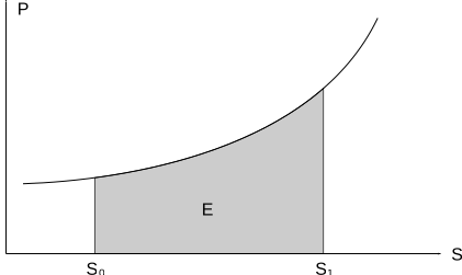 An example supply versus price graph. The area below the curve is equal to the amount of ETH that must be spent to increase the supply from to , or that is going to be received when tokens are unbonded.
Inside a transaction, the price paid/received per token is not constant and depends on the amount that is bonded or unbonded. This complicates the calculations.
Let’s say for an initial supply of , we want to bond tokens which are added to the new supply . The ETH that must be spent for this bonding is defined as
which is illustrated in the figure above. If one wanted to unbond tokens, the upper limit for the integral would be and the lower , with E corresponding to the amount of ETH received for the unbonding.
Linear Curves
A linear relationship for the bonding curves are defined as
where is the initial price of the token and is the price increment per token.
Bonding Tokens
Let us have ETH which we want to bond tokens with. Substituting into the integral above with the limits , we obtain in terms of the tokens that we want to bond:
where is the supply before the bonding. Solving this for , we obtain the tokens received in a bonding as a function of the supply and ETH spent:
Unbonding Tokens
Let us have T tokens which we want to unbond for ETH. Unbonding tokens decreases the supply from to , which we apply as limits for the above integral and obtain:
Breaking Even in PoWH3D
PoWH3D is one of the applications of bonding curves with a twist: 1/10th of every transaction is distributed among token holders as dividends. When you bond tokens with ETH, you receive worth of tokens and is distributed to everybody else in proportion to the amount they hold.
This means you are at a loss when you bond P3D (the token used by PoWH3D). If you were to unbond immediately, you would only receive 81% of your money. Given the situation, one wonders when exactly one can break even with their investment. The activity in PoWH3D isn’t deterministic; nonetheless we can deduce sufficient but not necessary conditions for breaking even in PoWH3D.
Sufficient Bonding
Let us spend ETH to bond tokens at supply . The following calculations are done with the assumption that the tokens received
are small enough to be neglected, that is and . In other words, this only holds for non-whale bondings.
Then let others spend ETH to bond tokens and raise the supply to . The objective is to find an large enough to earn us dividends and make us break even when we unbond our tokens at . We have
Our new share of the P3D pool is and the dividends we earn from the bonding is equal to
Then the condition for breaking even is
This inequality has a lengthy analytic solution which is impractical to typeset. The definition should be enough:
}\left\{\frac{9}{10} E(S_2, T_1) + \frac{1}{10}\frac{T_1}{S_2}E_2 = E_1\right\}and
can be obtained from the source of this page in JavaScript from the function
sufficient_bonding. The function involves many power and square operations and may yield inexact results for too high values of or too small values off , due to insufficient precision of the underlying math functions. For this reason, the calculator is disabled for sensitive input.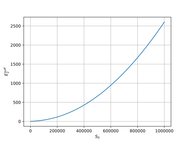 versus for .
The relationship between the initial supply and sufficient bonding is roughly quadratic, as seen from the graph above. This means that the difficulty of breaking even increases quadratically as more people bond into P3D. As interest in PoWH3D saturates, dividends received from the supply increase decreases quadratically.
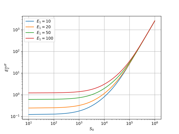 Logarithmic plot of versus for changing values of .
The relationship is not exactly quadratic, as seen from the graph above. The function is sensitive to for small values of .
Sufficient Unbonding
Let us spend ETH to bond tokens at supply and receive tokens.
Then let others unbond P3D to lower the supply to . The objective is to find a large enough to earn us dividends and make us break even when we unbond our tokens at . We have
Our new share of the P3D pool is and the dividends we earn from the bonding is equal to
Then the condition for breaking even is
Similar to the previous section, we have
}\left\{\frac{9}{10} E(S_2, T_1) + \frac{1}{10}\frac{T_1}{S_2} E(S_2, T_2) = E_1\right\}and
can be obtained from the function
sufficient_unbonding.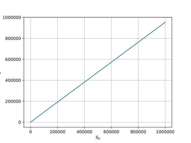 versus for .
The relationship between and is linear and insensitive to . Regardless of the ETH you invest, the amount of tokens that need to be unbonded to guarantee your break-even is roughly the same, depending on your entry point.
Calculator
Below is a calculator you can input and to calculate and .
For the default values above, we read this as:
For 100 ETH worth of P3D bonded at 3,500,000 supply, either a bonding of ~31715 ETH or an unbonding of ~3336785 P3D made by other people is sufficient to break even.
In order to follow these statistics, you can follow this site.
Conclusion
Bonding curve calculations can get complicated because the price paid per token depends on the amount of intended bonding/unbonding. With this work, I aimed to clarify the logic behind PoWH3D. Use the formulation and calculator at your own risk.
The above conditions are only sufficient and not necessary to break even. As PoWH3D becomes more popular, it gets quadratically more difficult to break even from a supply increase. PoWH3D itself doesn’t generate any value or promise long-term returns for its holders. However every bond, unbond and transfer deliver dividends. According to its creators, P3D is intended to become the base token for a number of games that will be built upon PoWH3D, like FOMO3D.