Entries for July 6, 2017
-

Duality of Vector Spaces
When I was learning about Continuum Mechanics for the first time, the covariance and contravariance of vectors confused the hell out of me. The concepts gain meaning in the context of Riemannian Geometry, but it was surprising to find that one doesn’t need to learn an entire subject to grasp the logic behind co-/contravariance. An intermediate knowledge of linear algebra is enough—that is, one has to be acquainted with the concept of vector spaces and one-forms.
The duality of co-/contravariance arises when one has to define vectors in terms of a non-orthonormal basis. The reason such terminology doesn’t show up in engineering education is that Cartesian coordinates are enough for most engineering problems. But every now and then, a complex problem with funky geometrical requirements show up, like one that requires measuring distances and areas on non-flat surfaces. Then you end up with dual vector spaces. I’ll try to give the basics of duality below.
Definition: Let be a finite-dimensional real vector space. The space , defined as the the space of all one-forms , is called the dual space to .
Let be a basis of . Any vector can be written in terms of as
with the components . For any , we can define the -th component by a one-form as
These elements are linear and thus are in the space 1. Given any basis , we call the basis of dual to . The fact that really is a basis of can be proved by showing that are linearly independent. Then has the following representation
Instead of , it is practical to denote the components of as , lightface of the same symbol with a raised index corresponding to the raised index of the dual basis:
In fact, this convention is more compatible with the symmetry caused by the duality. This point will be more clear after the introduction of dual basis representation of one-forms.
Proposition: Each can be identified by its action on the basis :
Proof: For any , must give , the -th component of . Setting , one sees that when , and is zero otherwise.
Geometrically, (5) implies that a basis vector is perpendicular to all the dual basis vectors, except its own dual.
Dual Basis Representation of One-Forms
Let be a one form in with the corresponding dual basis . Then similar to a vector, has the following representation
where the components of the one-form are defined as
Proof: We substitute (3) and obtain
using ‘s linearity.
Notation: Let be a finite-dimensional real vector space. For and
denotes the action of on , and is called a natural pairing or dual pairing between a vector space and its dual. It is of the essence to understand that does not denote an inner product in ; that is, means .
With this notation, (3) can be written as
and (5) as
Using the convention that are column vectors and are row vectors, (11) can be rearranged in the following manner
which can be used to compute a dual basis.
Example: Given a two-dimensional vector space with a basis , , we use (12) to compute
and obtain the dual basis vectors as and . The result is given in the following figure,
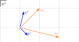
where one can see that , .
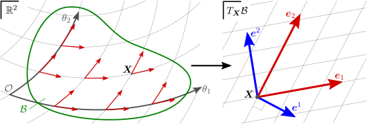 A body embedded in with curvilinear coordinates.
Every point at has an associated two-dimensional vector space,
called 's tangent space at , denoted . The basis
corresponding to coordinates are not necessarily
orthogonal and can admit corresponding duals , due to
curvilinearity.
The coordinates appear to be affine at the point's immediate vicinity,
and thus in the tangent space.
A body embedded in with curvilinear coordinates.
Every point at has an associated two-dimensional vector space,
called 's tangent space at , denoted . The basis
corresponding to coordinates are not necessarily
orthogonal and can admit corresponding duals , due to
curvilinearity.
The coordinates appear to be affine at the point's immediate vicinity,
and thus in the tangent space.
The introduction of the dual space allows us to reinterpret a one-form as an object residing in the dual space. In fact, the canonical duality states that every vector can be interpreted as a functional on the space via
-
Despite being denoted with bold letters, one-forms should not be confused with vectors. ↩
-