Entries for July 2017

Equipping a vector space with an inner product results in a natural isomorphism $\CV\to\CV^\ast$, where the metric tensor can be interpreted as the linear mapping $\Bg:\CV\to\CV^\ast$ and its inverse $\Bg\inv:\CV^\ast\to\CV$.

Notation: Given two real vector spaces $\CV$ and $\CW$, we denote their inner products as $\dabrn{\cdot,\cdot}_{\CV}$ and $\dabrn{\cdot,\cdot}_{\CW}$ respectively. Given vectors $\Bv\in\CV$ and $\Bw\in\CW$, we define their lengths as

Regarding $\CV$ and $\CW$,

1. their bases are denoted $\cbrn{\BE_A}$ and $\cbrn{\Be_a}$,
2. their dual bases are denoted $\cbrn{\BE^A}$ and $\cbrn{\Be^a}$,
3. their metrics are denoted $\BG$ and $\Bg$ with the components $G_{AB}=\dabrn{\BE_A,\BE_B}_{\CV}$ and $g_{ab}=\dabrn{\Be_a,\Be_b}_{\CW}$,

respectively. Here, the indices pertaining to $\CV$ are uppercase $(ABC\dots)$ and the indices pertaining to $\CW$ are lowercase $(abc\dots)$.

Definition: Let $\BP:\CV\to\CW$ be a linear mapping. Then the transpose, or adjoint of $\BP$, written $\BP\tra$, is the linear mapping

for all $\Bv\in\CV$ and $\Bw\in\CW$. Carrying out the products,

For arbitrary $\Bv$ and $\Bw$,

from which we can obtain the components of the transpose as

If $\BB:\CV\to\CV$ is a linear mapping, it is called symmetric if $\BB=\BB\tra$.

Definition: Let $\BP:\CV\to\CW$ be a linear mapping. Then the dual of $\BP$ is a metric independent mapping

defined through natural pairings for all $\Bv\in\CV$ and $\Bbeta\in\CW^\ast$. Carrying out the products,

For arbitrary $\Bv$ and $\Bbeta$, we obtain the components of the dual mapping as

To fully appreciate the symmetry that originates from the duality, we can think of not just the mappings between $\CV$ and $\CW$, but also between their dual spaces. To this end we can enumerate four mappings corresponding to $\cbr{\CV,\CV^\ast}\to\cbr{\CW,\CW^\ast}$ and their duals, corresponding to $\cbr{\CW,\CW^\ast}\to\cbr{\CV,\CV^\ast}$. Their definitions can be found in the table below.

The commutative diagrams pertaining to these mappings can be found in the figure below

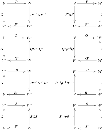
Commutative diagrams involving the linear mappings $\BP,\BQ,\BR,\BS$ and their dual $\BP^\ast,\BQ^\ast,\BR^\ast,\BS^\ast$ based on the metrics $\BG$ and $\Bg$ of $\CV$ and $\CW$.

The assignment of an inner product to a non-degenerate and finite-dimensional vector space $\CV$, results in emergence of the natural isomorphism to its dual $\CV\to\CV^\ast$, which means that the morphisms $\CV\to\CV^\ast$ and $\CV^\ast\to\CV$ are of the same structure and one is the inverse of the other. The notion of naturality (of an isomorphism) becomes most clear in the context of category theory; however it should be sufficient for now to say that a natural isomorphism between a vector space an its dual is one that is basis-independent. As the origin of the isomorphism, the inner product is encapsulated in an object called the metric, defined below, in order to make the resulting symmetry of the mappings more obvious.

In the context of differential geometry, the metric object is used synonymously with the inner product of a vector space. More specifically, the metric tensor

of a real vector space $\CV$ is an object whose components contain the information necessary to linearly transform a vector to its covector. This operation is denoted by the symbol $\flat$ and reads

We simply define the one-form $\Bv^\flat$ as

We input the basis vectors $\Be_a$

and define the components of the metric tensor as

We then simply say that the operator $\flat$ denotes an index lowering¹ through

Moreover, we can define the inverse of the metric tensor as

The operation of transforming a covector to its corresponding vector is denoted by the symbol $\sharp$ and reads

Here, the vector corresponding to the covector $\Balpha$ is denoted $\Balpha^\sharp$ and reads

We input the dual basis vectors $\Be^a$

and define the components of the inverse metric $\Bg\inv$ as

Then the operator $\sharp$ denotes an index raising through

In some literature, the natural isomorphism $\CV\to\CV^\ast$ is called the musical isomorphism—which is also the origin of the notation introduced above—because the process of transforming a vector to its dual space and a covector to the original space is analogous to lowering and raising notes.

With the given definition of the metric, we can elaborate on the advantage of denoting inner products of different objects with different symbols. Whereas $\abrn{\cdot,\cdot}$ always denotes a natural pairing between a vector space and its dual, one can write $\dabrn{\cdot,\cdot}_{\CV}:\CV\times\CV\to\IR$ to denote an inner product of vectors and $\dabrn{\cdot,\cdot}_{\CV^\ast}:\CV^\ast\times\CV^\ast\to\IR$ to denote an inner product of covectors. Using the metric, we can link these notations as

for all $\Bv,\Bw\in\CV$ and $\Balpha,\Bbeta\in\CV^\ast$. Similarly,

Despite the symmetricity of the inner product, we choose to think of the first operand as a vector and the second as a covector in a natural pairing, as a convention.

The metric tensor has the following properties:

• For orthonormal bases, the metric tensor equals the identity tensor, that is, $g_{ij}=\delta_{ij}$.
• The diagonal terms equal to the square of the lengths of the basis vectors, that is, $g_{ii}=\Norm{\Be_i}^2$ (no summation).
• The off-diagonal terms are zero if the basis vectors are orthogonal. Specifically, $g_{ij}=0$ iff $\Be_i$ and $\Be_j$ are orthogonal.

When I was learning about Continuum Mechanics for the first time, the covariance and contravariance of vectors confused the hell out of me. The concepts gain meaning in the context of Riemannian Geometry, but it was surprising to find that one doesn’t need to learn an entire subject to grasp the logic behind co-/contravariance. An intermediate knowledge of linear algebra is enough—that is, one has to be acquainted with the concept of vector spaces and one-forms.

The duality of co-/contravariance arises when one has to define vectors in terms of a non-orthonormal basis. The reason such terminology doesn’t show up in engineering education is that Cartesian coordinates are enough for most engineering problems. But every now and then, a complex problem with funky geometrical requirements show up, like one that requires measuring distances and areas on non-flat surfaces. Then you end up with dual vector spaces. I’ll try to give the basics of duality below.

Definition: Let $\CV$ be a finite-dimensional real vector space. The space $\CV^\ast = \CL(\CV,\IR)$, defined as the the space of all one-forms $\Balpha:\CV\to\IR$, is called the dual space to $\CV$.

Let $B=\cbr{\Be_1,\dots,\Be_n}$ be a basis of $\CV$. Any vector $\Bv\in\CV$ can be written in terms of $B$ as

with the components $a_1,\dots,a_n\in\IR$. For any $i=1,\dots,n$, we can define the $i$-th component $a_i$ by a one-form as

These elements are linear and thus are in the space $\CL(\CV,\IR)$¹. Given any basis $B=\setveci{\Be}$, we call $B^\ast = \setveciup{\Be}$ the basis of $\CV^\ast$ dual to $B$. The fact that $B^\ast$ really is a basis of $\CV^\ast$ can be proved by showing that $\Be^i$ are linearly independent. Then $\Bv$ has the following representation

Instead of $a_i$, it is practical to denote the components of $\Bv$ as $v^i$, lightface of the same symbol with a raised index corresponding to the raised index of the dual basis:

In fact, this convention is more compatible with the symmetry caused by the duality. This point will be more clear after the introduction of dual basis representation of one-forms.

Proposition: Each $\Be^i \in \CL(\CV,\IR)$ can be identified by its action on the basis $B$:

Proof: For any $\Bv\in\CV$, $\Be^i(\Bv)$ must give $v^i$, the $i$-th component of $\Bv$. Setting $\Bv = \Be_j$, one sees that $\Be^i(\Bv)=v^i = 1$ when $i=j$, and is zero otherwise.

Geometrically, (5) implies that a basis vector is perpendicular to all the dual basis vectors, except its own dual.

Dual Basis Representation of One-Forms

Let $\Balpha$ be a one form in $\CV^\ast$ with the corresponding dual basis $\setveciup{\Be}$. Then similar to a vector, $\Balpha$ has the following representation

where the components of the one-form $\Balpha$ are defined as

Proof: We substitute (3) and obtain

using $\Balpha$‘s linearity.

Notation: Let $\CV$ be a finite-dimensional real vector space. For $\Bv\in\CV$ and $\Balpha\in\CV^\ast$

denotes the action of $\Balpha$ on $\Bv$, and is called a natural pairing or dual pairing between a vector space and its dual. It is of the essence to understand that $\abrn{\cdot,\cdot}$ does not denote an inner product in $\CV$; that is, $\abr{\Bv,\Balpha}$ means $\Balpha(\Bv)$.

With this notation, (3) can be written as

and (5) as

Using the convention that $\Be_i$ are column vectors and $\Be^i$ are row vectors, (11) can be rearranged in the following manner

which can be used to compute a dual basis.

Example: Given a two-dimensional vector space $\CV$ with a basis $\Be_1=[2,-0.5]\tra$, $\Be_2=[1,1]\tra$, we use (12) to compute

and obtain the dual basis vectors as $\Be^1=[0.4,-0.4]$ and $\Be^2=[0.2,0.8]$. The result is given in the following figure,

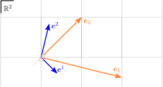
where one can see that $\Be_1\perp\Be^2$, $\Be^1\perp\Be_2$.

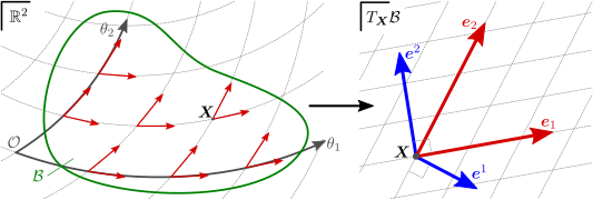
A body $\CB$ embedded in $\IR^2$ with curvilinear coordinates. Every point $\CP$ at $\BX$ has an associated two-dimensional vector space, called $\CB$'s tangent space at $\BX$, denoted $\tang_{\BX}\CB$. The basis $\Be_i$ corresponding to coordinates $\theta_i$ are not necessarily orthogonal and can admit corresponding duals $\Be^i$, due to curvilinearity. The coordinates appear to be affine at the point's immediate vicinity, and thus in the tangent space.

The introduction of the dual space allows us to reinterpret a one-form $\Balpha$ as an object residing in the dual space. In fact, the canonical duality $\CV^{\ast\ast}=\CV$ states that every vector $\Bv$ can be interpreted as a functional on the space $\CV^\ast$ via