Entries for 2017
-

Nonlinear Finite Elements
This post builds on the formulations I showed in my previous posts by introducing their nonlinear versions.
In a typical nonlinear problem, the variational setting leads to the weak formulation
Find such that
for all where the semilinear form is nonlinear in terms of and linear in terms of .
We linearize :
Equating (2) to zero yields a linear system in terms of
where
We can compute the components of the matrices and vectors according to (3)
Then the update vector is obtained by solving
Letting be the difference between consequent iterates, we obtain the update equation as
Example: Nonlinear Poisson’s Equation
Consider the following nonlinear Poisson’s equation
The weak formulation reads
Find such that
for all where .
Applying integration by parts and divergence theorem on the left-hand side
Thus we have the semilinear form
The linearized version of this problem is then with (4)
and the matrix and vector components are with (5)
where the previous solution and its gradient are computed as
Nonlinear Time-Dependent Problems
In the case of a nonlinear time-dependent problem, we have the following weak form:
Find such that
for all and where is a semilinear form.
Discretization yields the following nonlinear system of equations
where
Explicit Euler Scheme
We discretize in time with the finite difference and linearity allows us to write
\begin{equation} \boxed{ m(\dot{u}, v; t) \approx \frac{1}{\Delta t} [m(u_{n+1}, v; t_{n+1}) - m(u_n, v; t_n)] } \label{eq:discretetimedependent1} \end{equation}
We discretize the variational forms in time according to \eqref{eq:discretetimedependent1}, and evaluate the remaining terms at :
The corresponding system of equations is
where . This yields the following update equation
For a time-independent , this becomes
Implicit Euler Scheme
For the implicit scheme, we evaluate the remaining terms at and let the result be equal to
We will hereon replace with for brevity. The update of this nonlinear system requires the linearization of :
We thus have the following linear setting for the Newton update :
where
Discretization yields
where
The Newton update is rendered
which is repeated until the solution for the next timestep converges to a satisfactory value.
Nonlinear Coupled Problems
For a nonlinear coupled problem, the weak formulation is as follows
Find , such that
for all , where , are nonlinear in terms of and and linear in terms of and .
We linearize the semilinear forms about the nonlinear terms:
where the evaluations take place at and .
Equating the linearized residuals to zero, we obtain a linear system of the form
with the bilinear forms , , , and the linear forms , which are defined as
Discretizing as done in the previous section, we obtain the following linear system of equations
whose solution yields the update values and . Thus the Newton update equations are
Example: Cahn-Hilliard Equation
The Cahn-Hilliard equation describes the process of phase separation, by which the two components of a binary fluid spontaneously separate and form domains pure in each component. The problem is nonlinear, coupled and time-dependent. The IBVP reads
where
and . Here,
- is the scalar variable for concentration,
- is the scalar variable for the chemical potential,
- is the function representing chemical free energy,
- is a second-order tensor describing the mobility of the chemical,
- is a second-order tensor describing both the interface thickness and direction of phase transition.
The fourth-order PDE governing the problem can be formulated as a coupled system of two second-order PDEs with the variables and , as demonstrated in (35) and (36).
The weak formulation then reads
Find , such that
for all , and .
We discretize in time implicitly with . We also denote the values for the next timestep and as and for brevity. Using integration-by-parts, the divergence theorem, and the given boundary conditions, we arrive at the following nonlinear forms
which is a nonlinear coupled system of the form (29).
We linearize the forms according to (30) and obtain the following variations
We substitute basis functions and obtain our system matrix and vectors
which constitute the system
Solution yields the update values and . The Newton update equations are then
The system is solved for and at each to obtain the evolutions of the concentration and chemical potential.
-
Coupled Finite Elements
In this post, I’ll introduce the FE formulation of a generalized linear and coupled weak form. Said weak formulation has the form
Find , such that
for all , where , , , are bilinear forms and , are linear forms.
Here, the objective is to solve for the two unknown functions and . One can also imagine an arbitrary degree of coupling between variables with equations.
We introduce the following discretizations
where the corresponding number of shape functions are and , respectively.
Substituting the discretizations in (1), we obtain two linear systems of equations
for and .
We write this system as
where the components of given matrices and vectors are defined as
Solution of (4) yields the unknown vectors and .
-
Time-Dependent Finite Elements
Time dependent problems are commonplace in physics, chemistry and many other disciplines. In this post, I’ll introduce the FE formulation of linear time-dependent problems and derive formulas for explicit and implicit Euler integration.
The weak formulation of a first order time-dependent problem reads:
Find such that
for all and .
We can convert (1) into a system of equations
where the components of the matrices and vectors involved are calculated as
If we further discretize in time with the finite difference , linearity allows us to write
This reflects on the system as
Here, , and vice versa for and .
Explicit Euler Scheme
For the explicit Euler scheme, we substitute evaluate the remaining terms at
The corresponding system is
The update equation becomes
If is time-independent, that is , we have
Implicit Euler Scheme
For the implicit Euler scheme, we substitute evaluate the remaining terms at
The corresponding system is
The update equation becomes
If is time-independent, one can just substitute .
Example: Reaction-Advection-Diffusion Equation
The IBVP of a linear reaction-advection-diffusion problem reads
where ,
- is a second-order tensor describing the diffusivity of ,
- is a vector describing the velocity of advection,
- is a scalar describing the rate of reaction,
- and is a source term for .
The weak formulation is then
Find such that
for all and .
We have the following integration by parts relationships:
for the diffusive part and
for the advective part. The canceled terms are due to divergence theorem and the fact that on the boundary. Then our variational formulation is of the form (1) where
From these forms, we obtain the following system matrices and vector
where is constant through time.
-
Vectorial Finite Elements
Many initial boundary value problems require solving for unknown vector fields, such as solving for displacements in a mechanical problem. Discretization of weak forms of such problems leads to higher-order linear systems which need to be reshaped to be solved by regular linear solvers. There are also more indices involved than a scalar problem, which can be confusing. In this post, I’ll try to elucidate the procedure by deriving for a basic higher-order system and giving an example.
The weak formulation of a linear vectorial problem reads
Find such that
for all .
Discretizations of vectorial problems requires the expansion of vectorial quantities as linear combinations of the basis vectors :
where are the components corresponding to the basis vectors and . Here, we chose Cartesian basis vectors for simplicity.
We can therefore express its discretization as
Substituting discretized functions in the weak formulation, we obtain
and
We define the following arrays
Hence we can express the linear system
as
For arbitrary , this yields the following system of equations
for and .
We reshape this higher-order system as shown in the previous post Reshaping Higher Order Linear Systems:
by defining a map that maps original indices to the reshaped indices
where we used 1-based indexing of the arrays. We set
and write
The inverse index mapping can be obtained as shown in the previous post.
Example: Linear Elasticity
Our initial-boundary value problem is
The weak formulation reads
Find such that
for all where .
We apply integration by parts on the left-hand side
and apply the divergence theorem to the first resulting term:
Substituting the linear stress , we obtain the following variational forms:
We have the following discretizations of the unknown function and test function
With the given discretizations, the matrix corresponding to (18) can be calculated as
and finally obtain
The vector corresponding to (19) is calculated as
which yields
-
Reshaping Higher Order Linear Systems
In vectorial problems, we end up with linear systems of higher order, such as
for and .
These systems cannot be solved readily with existing software. In order to be able to solve them with existing software, we need to reshape them by defining a matrix of matrices and vector of vectors and :
This allows us to express the linear system as
Here, we reshape the system by defining a map that maps original indices to the reshaped indices
where we used 1-based indexing of the arrays. We set
and write
For reference, the inverse of the index mapping reads
Thus, we have for our reshaped indices,
Expressed as a regular linear system (3), the higher-order system (1) can be solved with a linear solver such as LAPACK.
-
Linear Finite Elements
Beginning with this post, I’ll be publishing about the basics of finite element formulations, from personal notes that accumulated over the years. This one is about linear and scalar problems which came to be the “Hello World” for FE. Details regarding spaces and discretization are omitted for the sake of brevity. For those who want to delve into theory, I recommend “The Finite Element Method: Theory, Implementation, and Applications” by Larson and Bengzon.
The weak formulation of a canonical linear problem reads
Find such that
for all where is a bilinear form and is a linear form.
We define the discretization of as
The discretization is a linear combination of basis functions and corresponding scalars , so that is a subset of . The discretization of (1) then reads
We then have
Using the linearity properties,
we obtain
For arbitrary test function values , we can express (6) as a system of equations
for . If we expand the summations as
we can see that the terms with constitute a matrix and the terms with constitute a vector , allowing us to write
where we chose to express the unknown coefficients as a vector .
\It can be seen that the components of the and are defined as
we can express the linear system as
Note that with the given definitions, (7) becomes
Example: Poisson’s Equation
In the weak form of Poisson’s equation
The weak formulation reads
Find such that
for all where .
Applying integration by parts and divergence theorem on the left-hand side
We have the following variational forms:
Following (7), we can calculate the stiffness matrix as
where we have defined the gradient of the basis functions as
Similarly, we integrate the force term into a vector as
-
Balance Laws
Calculus is all about relating the change in one quantity to another quantity.
Imagine it this way: You have a box full of marbles, and you decide to put some more in. is the variable representing the amount of marbles, while is the variable representing the amount of marbles that you put in. If you had marbles at the beginning, you have
marbles following your action. This is the most fundamental algebraic pattern that characterizes balance laws.
Take the first law of thermodynamics for example—a.k.a. balance of energy. We have
where is the internal energy of a closed system, is the amount of heat supplied to the system, and is the amount of work done on the system on its surroundings. Here, and . Despite having three quantities, it is the combined effect of two which is related to the remaining quantity. Balance laws derived by physicists and chemists can get quite complex and hard to understand.
It’s always that the change in one quantity is related to the combined effect of remaining quantities. Keeping separate track of your main variable and affecting variables that compose gives you a mental model which helps you remember and even build your own balance laws.
Introducing Time
Let be a function of time. We can rewrite the equation in terms of the change in in a time period :
where the new variable represents the change in quantity in amount of time. In our previous analogy, is the amount of marbles put in, say, a minute. As , we have
This prototypical balance law allows us to relate the rates of change of quantities.
Let’s introduce time into the balance of energy. The equation becomes
where the new quantities and are called thermal power and mechanical power, representing the thermal and mechanical work done on the system per unit time, respectively. Given power functions and initial conditions, integrating them would give us the evolution of the internal energy through time.
Introducing Space
Let’s say we are not satisfied with an abstract box where the amount of stuff that goes in is measured automatically. We want to write a balance law over different shapes of bodies and we need to specify exactly where the stuff goes in and out.
To do that, we need to rephrase our laws to work over a continuous domain. The branch of physics that focuses on such problems is called continuum mechanics.
We introduce our spatial domain and its boundary . Our quantities now vary over both space and time, so we need to integrate them over the whole domain in order to relate them:
where
- is the variable representing the main continuous quantity,
- is the variable representing the rate of change of the quantity inside the domain,
- and is the variable representing the negative rate of change of the quantity on the boundary of the domain—negative due to surface normals having outward direction by definition.
Notice that when we introduce space, our prototypical balance law needs an additional vectorial quantity, . In physical laws, one needs to differentiate actions inside a body from actions on the surface of the body. That’s because one is over a volume and the other over an area, and they have to be integrated separately.
The area integral is actually a flux where the vectorial quantity is penetrating the surface with a given direction. Given that it’s positive when stuff exits the domain, it’s called the efflux of the underlying quantity. Similarly, we name the rate of change field as the supply of the underlying quantity, because it being positive results in an increase.
The idea is to get rid of the integrals by a process called “localization”. In order to localize, we have to convert the surface integral into a volume integral using the divergence theorem:
Assuming doesn’t move, we can also write
Collecting the results, we have
Notice that all integrals are over now. This allows us to make the balance law more strict by enforcing it point-wise:
This is the localized version of the prototypical balance law that is used everywhere in continuum mechanics. Unfortunately, I can’t give the energy balance example, because it would require too many additional definitions. For that, I recommend the excellent Mathematical Foundations of Elasticity by Marsden and Hughes.
Conclusion
In physics and chemistry, one shouldn’t blindly memorize formulas, but try to see the underlying logic. In this case, I tried to elucidate balance laws, which all build upon the same algebraic and geometrical concepts. I went from discrete to continuous by introducing time and space to the equations, which became more complex but retained the same idea: putting things in a box and trying to calculate how that changes the contents.
-
Taylor and Volterra Series
In the theory of computational mechanics, there are a few operations used that are not taught in Calculus 101, which can be confusing without taking a lecture in calculus of variations. One of them is taking variations (a.k.a. Gateaux derivatives), akin to taking directional derivatives, but with functions of functions called functionals.
You need to take variations when you are linearizing a nonlinear problem for the purpose of solving with a numerical scheme. Linearization is the process of expanding a function or functional into a series, and discarding terms that are of order higher than linear—i.e. quadratic, cubic, quartic, etc. These expansions are called Taylor for functions, and Volterra for functionals.
Taylor Series
A function can be expanded about a point as a power series:
Letting be a perturbation from the expansion point , that is , the series can also be phrased as follows
This is what is taught in Calculus 101 and everyone knows. Now for the part that you may have missed:
Variation
Let be the space of functions . The variation of a functional is defined as
where is called the perturbation of the variation. This operation is analogous to taking the directional derivative of a function.
Shorthand notation
When working with variational formulations, writing out variations can be a bit of a hassle if there are many symbols involved. Therefore we use the following shorthand for variations:
Here, we assume that there is no chance of confusing the varied function or perturbation. We use this shorthand in contexts where the perturbation does not play an important role.
The shorthand for evaluation is
where there is no risk of confusion for .
Volterra Series
Let be the space of functions . Analogous to the Taylor series, a functional can be expanded about a point as a power series:
where is the perturbation of the expansion. This is called the Volterra series expansion of . Verbally, the Volterra series expansion of a functional about a function is the infinite sum of the variations of the functional with increasing degree, evaluated at that function, each divided by the factorial of the degree.
In shorthand notation, the expansion is rendered
To me, there is an elegance in (7) that is not reflected in (2) or (6).
-
Isomorphisms in Linear Mappings between Vector Spaces
Equipping a vector space with an inner product results in a natural isomorphism , where the metric tensor can be interpreted as the linear mapping and its inverse .
Notation: Given two real vector spaces and , we denote their inner products as and respectively. Given vectors and , we define their lengths as
Regarding and ,
- their bases are denoted and ,
- their dual bases are denoted and ,
- their metrics are denoted and with the components and ,
respectively. Here, the indices pertaining to are uppercase and the indices pertaining to are lowercase .
Definition: Let be a linear mapping. Then the transpose, or adjoint of , written , is the linear mapping
for all and . Carrying out the products,
For arbitrary and ,
from which we can obtain the components of the transpose as
If is a linear mapping, it is called symmetric if .
Definition: Let be a linear mapping. Then the dual of is a metric independent mapping
defined through natural pairings for all and . Carrying out the products,
For arbitrary and , we obtain the components of the dual mapping as
To fully appreciate the symmetry that originates from the duality, we can think of not just the mappings between and , but also between their dual spaces. To this end we can enumerate four mappings corresponding to and their duals, corresponding to . Their definitions can be found in the table below.
Mappings
Duals
Tensors , , and as linear mappings (top), and their duals , , and (bottom). In the respective tables, the first row displays the tensor spaces, basis vectors and components of the subsequent mappings, and the second and third row display the representations of the tensor as linear and bilinear mappings respectively. The results of the mappings are given in the mapping, matrix and index representations respectively. The mappings are over vectors , and one-forms , . The commutative diagrams pertaining to these mappings can be found in the figure below
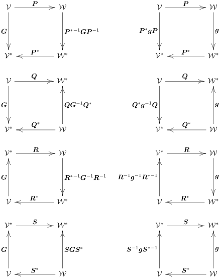 Commutative diagrams involving
the linear mappings and
their dual
based on the metrics and
of and .
Commutative diagrams involving
the linear mappings and
their dual
based on the metrics and
of and .
-
Metrics and Natural Isomorphisms
The assignment of an inner product to a non-degenerate and finite-dimensional vector space , results in emergence of the natural isomorphism to its dual , which means that the morphisms and are of the same structure and one is the inverse of the other. The notion of naturality (of an isomorphism) becomes most clear in the context of category theory; however it should be sufficient for now to say that a natural isomorphism between a vector space an its dual is one that is basis-independent. As the origin of the isomorphism, the inner product is encapsulated in an object called the metric, defined below, in order to make the resulting symmetry of the mappings more obvious.
In the context of differential geometry, the metric object is used synonymously with the inner product of a vector space. More specifically, the metric tensor
of a real vector space is an object whose components contain the information necessary to linearly transform a vector to its covector. This operation is denoted by the symbol and reads
We simply define the one-form as
We input the basis vectors
and define the components of the metric tensor as
We then simply say that the operator denotes an index lowering1 through
Moreover, we can define the inverse of the metric tensor as
The operation of transforming a covector to its corresponding vector is denoted by the symbol and reads
Here, the vector corresponding to the covector is denoted and reads
We input the dual basis vectors
and define the components of the inverse metric as
Then the operator denotes an index raising through
In some literature, the natural isomorphism is called the musical isomorphism—which is also the origin of the notation introduced above—because the process of transforming a vector to its dual space and a covector to the original space is analogous to lowering and raising notes.
With the given definition of the metric, we can elaborate on the advantage of denoting inner products of different objects with different symbols. Whereas always denotes a natural pairing between a vector space and its dual, one can write to denote an inner product of vectors and to denote an inner product of covectors. Using the metric, we can link these notations as
for all and . Similarly,
Despite the symmetricity of the inner product, we choose to think of the first operand as a vector and the second as a covector in a natural pairing, as a convention.
The metric tensor has the following properties:
- For orthonormal bases, the metric tensor equals the identity tensor, that is, .
- The diagonal terms equal to the square of the lengths of the basis vectors, that is, (no summation).
- The off-diagonal terms are zero if the basis vectors are orthogonal. Specifically, iff and are orthogonal.
-
In musical notation, the flat symbol is used to lower a note by one semitone, whereas the sharp symbol is used to raise a note by one semitone. It is recommended to pronounce as v-flat and alpha-sharp. ↩
-
Duality of Vector Spaces
When I was learning about Continuum Mechanics for the first time, the covariance and contravariance of vectors confused the hell out of me. The concepts gain meaning in the context of Riemannian Geometry, but it was surprising to find that one doesn’t need to learn an entire subject to grasp the logic behind co-/contravariance. An intermediate knowledge of linear algebra is enough—that is, one has to be acquainted with the concept of vector spaces and one-forms.
The duality of co-/contravariance arises when one has to define vectors in terms of a non-orthonormal basis. The reason such terminology doesn’t show up in engineering education is that Cartesian coordinates are enough for most engineering problems. But every now and then, a complex problem with funky geometrical requirements show up, like one that requires measuring distances and areas on non-flat surfaces. Then you end up with dual vector spaces. I’ll try to give the basics of duality below.
Definition: Let be a finite-dimensional real vector space. The space , defined as the the space of all one-forms , is called the dual space to .
Let be a basis of . Any vector can be written in terms of as
with the components . For any , we can define the -th component by a one-form as
These elements are linear and thus are in the space 1. Given any basis , we call the basis of dual to . The fact that really is a basis of can be proved by showing that are linearly independent. Then has the following representation
Instead of , it is practical to denote the components of as , lightface of the same symbol with a raised index corresponding to the raised index of the dual basis:
In fact, this convention is more compatible with the symmetry caused by the duality. This point will be more clear after the introduction of dual basis representation of one-forms.
Proposition: Each can be identified by its action on the basis :
Proof: For any , must give , the -th component of . Setting , one sees that when , and is zero otherwise.
Geometrically, (5) implies that a basis vector is perpendicular to all the dual basis vectors, except its own dual.
Dual Basis Representation of One-Forms
Let be a one form in with the corresponding dual basis . Then similar to a vector, has the following representation
where the components of the one-form are defined as
Proof: We substitute (3) and obtain
using ‘s linearity.
Notation: Let be a finite-dimensional real vector space. For and
denotes the action of on , and is called a natural pairing or dual pairing between a vector space and its dual. It is of the essence to understand that does not denote an inner product in ; that is, means .
With this notation, (3) can be written as
and (5) as
Using the convention that are column vectors and are row vectors, (11) can be rearranged in the following manner
which can be used to compute a dual basis.
Example: Given a two-dimensional vector space with a basis , , we use (12) to compute
and obtain the dual basis vectors as and . The result is given in the following figure,
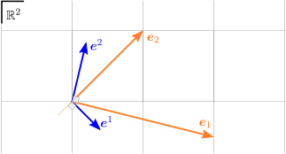
where one can see that , .
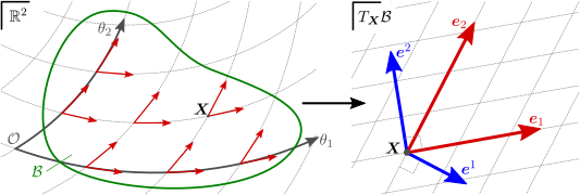 A body embedded in with curvilinear coordinates.
Every point at has an associated two-dimensional vector space,
called 's tangent space at , denoted . The basis
corresponding to coordinates are not necessarily
orthogonal and can admit corresponding duals , due to
curvilinearity.
The coordinates appear to be affine at the point's immediate vicinity,
and thus in the tangent space.
A body embedded in with curvilinear coordinates.
Every point at has an associated two-dimensional vector space,
called 's tangent space at , denoted . The basis
corresponding to coordinates are not necessarily
orthogonal and can admit corresponding duals , due to
curvilinearity.
The coordinates appear to be affine at the point's immediate vicinity,
and thus in the tangent space.
The introduction of the dual space allows us to reinterpret a one-form as an object residing in the dual space. In fact, the canonical duality states that every vector can be interpreted as a functional on the space via
-
Despite being denoted with bold letters, one-forms should not be confused with vectors. ↩
-