Entries for July 14, 2026

Note: this post is an AI-assisted write-up of the blackboard lecture Reiner Pope gave on Dwarkesh Patel’s podcast. Watch the original video: How GPT, Claude, and Gemini are actually trained and served (YouTube, 2h13m).¹

Pope is the CEO of the chip startup MatX and previously worked on TPU architecture at Google. With two rules of thumb (a roofline model of a GPU rack, and “set competing costs equal to each other”), he derives why batching makes tokens up to 1000x cheaper, why frontier models may be over-trained ~100x beyond Chinchilla-optimal, and how much of a lab’s serving stack you can reverse-engineer from its public API prices. The figures below are redrawn from the blackboard.

I have tried to stay faithful to the original throughout, converting the dialogue into prose and keeping all the numbers as stated. Any errors introduced in the conversion are mine.

The question that motivates everything

Dwarkesh opens with a pricing puzzle. Companies like Anthropic, OpenAI, and Cursor offer a “fast mode” that streams tokens at roughly 2.5x the speed for 6x the price. What is mechanically going on that makes this trade possible? Could you pay 100x more and go even faster? And could there be a “slow mode” where you wait minutes and pay much less?

Pope’s answer is that the dominant effect is batch size, and the rest of the lecture quantifies exactly what batching does to latency and cost. (A second effect, speculative decoding / multi-token prediction, is set aside.)

The whole analysis rests on two simplifications:

1. A roofline model of the hardware. For a cluster like an NVIDIA Blackwell NVL72 rack (72 GPUs), only two numbers matter: memory bandwidth and compute throughput (FLOPs).
2. Two numbers for the model. The time to operate on the weights, and the time to operate on the context (the KV cache).

The KV cache is the per-conversation state the model keeps in memory. During decode, each new token runs a full forward pass through all the weight matrices, and its attention mechanism looks back at an internal representation of every previous token. That stored representation is the KV cache, and reading it is dominated by memory fetches rather than matrix multiplies.

The two-line roofline

The time for one decode step is bounded below by whichever is slower, the memory system or the compute:

\[t \geq \max(t_{\mathrm{mem}},\; t_{\mathrm{compute}})\]

The compute side has to multiply a batch of $B$ tokens by all the active parameters:

\[t_{\mathrm{compute}} = \frac{B \cdot N_{\mathrm{active}}}{\mathrm{FLOPs}}\]

(The attention compute is ignored; it is small in comparison.) Note the distinction between active and total parameters: in a mixture-of-experts model like DeepSeek V3, about 37B parameters are active per token out of roughly 700B total.

The memory side has to fetch all the weights once per step, plus the KV cache of every sequence in the batch:

\[t_{\mathrm{mem}} \geq \frac{N_{\mathrm{total}} + B \cdot \mathrm{len}_{\mathrm{ctx}} \cdot \mathrm{bytes}_{\mathrm{tok}}}{\text{memory bytes/s}}\]

These two lines are enough to draw the latency picture:

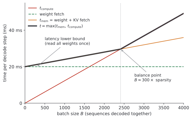
The weight fetch is a constant floor: no matter how small the batch, you must stream all total parameters from HBM into the chips once per token, and if you use all your memory bandwidth you cannot beat that. This is the latency lower bound, and it already answers the fast-mode question: for a given hardware configuration there is a floor on how fast tokens can come out, and paying more only helps until you hit it.

Cost is a different plot. Renting the GPUs for one step costs the same regardless of batch size, but the step produces $B$ tokens, so the cost per token is $t/B$:

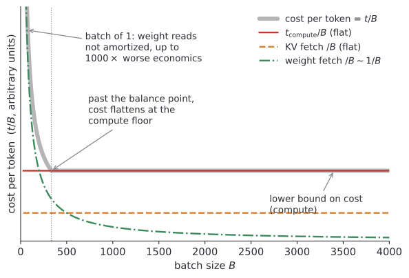
At batch size 1 the weight fetches are not amortized over anything and the economics are up to a thousand times worse. As the batch grows, the weight-fetch hyperbola vanishes and the compute term becomes a hard cost floor. This also answers the “slow mode” question: a hypothetical Claude Code Slow would live on that floor, and it would not be much cheaper than normal serving, because the compute and the KV fetches are unique to each request and cannot be amortized further.

The magic batch size

Where is the balance point where memory time equals compute time? Ignoring the KV term for a clean answer and equating the weight fetch with the weight multiply:

\[\frac{N_{\mathrm{total}}}{\text{mem BW}} = \frac{B \cdot N_{\mathrm{active}}}{\mathrm{FLOPs}} \quad\Longrightarrow\quad B = \frac{\mathrm{FLOPs}}{\text{mem BW}} \cdot \frac{N_{\mathrm{total}}}{N_{\mathrm{active}}}\]

The first factor is purely a hardware constant. Counted in FP4 multiplies (half a byte each), it comes out around 300 on most GPUs, and it has stayed roughly stable from A100 to H100 to B100 because FLOPs and memory bandwidth grew together. The second factor is the sparsity of the model. So:

\[B \gtrsim 300 \times \mathrm{sparsity}\]

For DeepSeek, which activates 32 of 256 experts (sparsity 8), that gives a batch of about 2,400 sequences. In practice people run double or triple that, since real-world efficiency is worse than the roofline. Including the KV fetch would push the optimal batch higher still. Remarkably, this result depends only on sparsity, never on model scale.

Trains departing every 20 milliseconds

How does a batch fill up with real users? Pope’s model is a train schedule. The server starts a new batch every ~20 ms whether or not it is full: any requests that are ready board the train, and a request that arrives just after departure waits for the next one. Worst-case queueing latency is therefore about 40 ms.

The 20 ms itself comes from a separate design principle: you want to read your entire HBM capacity once per forward pass, so the natural step time is capacity divided by bandwidth. On the Rubin generation that is 288 GB / 20 TB/s ≈ 15 ms, and the number has hovered around 20 ms across many HBM generations. There is no point going slower, because reading the read-only weights or the KV cache twice per token does nothing for you.

A batch of ~2,000 at ~64 steps per second is ~128,000 tokens per second per rack. Google has bragged about Gemini traffic in the hundreds of millions of tokens per second worldwide, so one rack’s economical batch is about one-thousandth of Gemini. That is the economy of scale in inference: real, but reachable by any serious provider.

Does sparsity hurt quality?

The roofline says sparsity is nearly free performance, so the follow-up is empirical: how much quality do you lose? From the paper “Unified Scaling Laws for Routed Language Models”, with an older MoE technique, a 64-expert model with 370M active parameters matched a dense 1.3B model. That is a 64x increase in total parameters for a 4x effective gain, a huge parameter cost for a modest efficiency win.

And yet from the systems side it is still nearly a pure win: the extra weight fetches amortize over a larger batch, so you keep increasing sparsity until you run out of simultaneous users. The real price is memory capacity, which is what the next sections are about.

Laying out a mixture of experts on a rack

An MoE layer has a router that sends each token to a small fraction of the experts (each expert being an ordinary MLP), an all-to-all “dispatch” of tokens to their experts, an all-to-all “combine” that sums the results, and a residual connection around the whole thing.

The standard practice is expert parallelism: different experts live on different GPUs. DeepSeek’s 256 experts on a Blackwell rack (using 64 of the 72 GPUs for divisibility) means 4 experts per GPU. Since the router’s decisions are data-dependent, any GPU may need to send tokens to any other GPU.

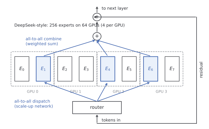
This all-to-all traffic pattern is a perfect fit for how a rack is wired. In NVIDIA’s design the GPUs sit on the outside of the rack and NVSwitches in the middle, with every GPU cabled to every switch, so any GPU reaches any other in two hops. This is the scale-up network (NVLink). Leaving the rack means taking the scale-out network through a NIC and a data-center switch, which is typically about 8x slower.

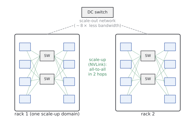
If you spread one expert layer across two racks, half of every all-to-all crosses the slow rack-to-rack boundary and becomes the bottleneck. So one rack bounds the size of an expert layer, and this is what has been driving interconnect domains bigger: Hopper had 8 GPUs in a scale-up domain, Blackwell 72, Rubin 500-something (some of that is Jensen math, but there is a genuine ~4x from a much harder rack design). The physical constraint is mundane: cable density. Doubling the GPUs in a rack literally doubles the density of cables that must be routed to the switches, against limits of space, weight, power, cooling, and the bend radius of the cables.

This is also a lens on model scaling history. GPT-4 (2023) was rumored to be over a trillion parameters, and models only clearly exceeded that scale once racks with tens of terabytes of fast memory arrived. Google’s TPU deployments have had very large scale-up domains for a long time, which may be part of why Gemini’s pre-training scaled successfully early. The summary: active parameters are limited by compute cost, and total parameters are limited by scale-up size.

Pipeline parallelism

Expert parallelism uses up one rack. To use more racks, the remaining options are data parallelism and pipeline parallelism (tensor parallelism has become irrelevant now that experts are small). Pipelining means putting different layers on different racks: a token flows through rack 0 for the first stage of layers, then hops to rack 1, and so on.

Is the hop a bottleneck? Compare the time spent on scale-up traffic to the time on scale-out traffic. Crossing racks sends each token once per stage, while inside the rack each token fans out to every activated expert, twice (dispatch and combine), for every layer in the stage:

\[\frac{t_{\text{scale-up}}}{t_{\text{scale-out}}} = \frac{1}{8} \cdot 2 \cdot (\text{activated experts}) \cdot (\text{layers per stage}) \;\geq\; 1\]

The 1/8 is the bandwidth ratio. With 8+ activated experts and a few layers per stage, the inequality is easily satisfied, so an entire pipeline of racks, one stage each, is communication-feasible.

Dwarkesh brings up Ilya’s remark that “as we now know, pipelining is not wise,” and the architectural constraints it imposes (e.g. Kimi’s attention to layers a few back is awkward to pipeline). Pope’s framing: pipelining is a massive hassle with real but narrow benefits. It saves no runtime at all (the memory fetches just happen on a different rack), but it divides the weight storage per rack, which matters if memory capacity is your constraint.

The catch is micro-batching. To keep four racks busy, you need four micro-batches in flight, each wrapping around for its next decode step as soon as it finishes:

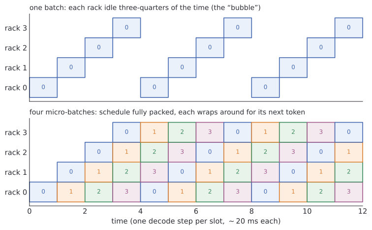
In inference this is natural and the bubble costs nothing; latency is identical to running unpipelined on one rack. In training there is a hard stop between the forward and backward passes of a batch, which creates a genuine bubble of idle time (the literature has zero-bubble and one-forward-one-backward schemes to interleave around it; as Dwarkesh notes, you could also mine Bitcoin in it):

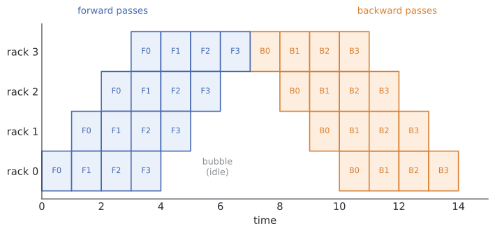
The training batch size itself is a trade-off: smaller batches are always better for ML convergence (fresher gradients), larger batches are better for systems throughput, and the optimum sits in between.

The memory wall and why the KV cache won’t shard

Here Dwarkesh raises the macro puzzle. Memory is the scarce commodity of the moment: Dylan Patel claims hyperscalers are spending half of their CapEx on memory, and consumer devices are getting squeezed. Yet the pipelining analysis just said racks have a memory surplus, since a trillion-parameter model needs only ~1 TB against a rack’s tens of TB. Why is Jensen shoving all that HBM in?

Write down the memory demand across the whole system:

\[C_{\mathrm{mem}} = N_{\mathrm{total}} + B \cdot \mathrm{len}_{\mathrm{ctx}} \cdot \mathrm{bytes}_{\mathrm{tok}}\]

Sharding across $E$ GPUs of expert parallelism and $P$ racks of pipelining, the per-GPU requirement is this divided by $E \cdot P$. But the global batch is (number of micro-batches) × (micro-batch size), and the number of micro-batches needed to fill the pipeline equals $P$, while the micro-batch size $b$ is pinned near $300 \times \mathrm{sparsity}$ by the roofline. Substituting $B = P \cdot b$, the $P$‘s cancel in the KV term:

\[c_{\mathrm{mem}}^{\text{per-GPU}} = \frac{N_{\mathrm{total}}}{E \cdot P} + \frac{b \cdot \mathrm{len}_{\mathrm{ctx}} \cdot \mathrm{bytes}_{\mathrm{tok}}}{E}\]

More pipeline stages keep shrinking the weight footprint, but the KV footprint per GPU stays constant: each extra stage requires proportionally more sequences in flight to stay busy. The KV cache can’t be amortized across the batch (it is unique per user), and it can’t be sharded across pipeline stages either. It loses on both fronts, and once you pipeline even a little, it becomes the dominant use of memory.

So what do labs actually run? Per the DeepSeek paper: expert parallelism up to the scale-up domain size, then very little pipelining (maybe none, maybe 2 stages so the weights aren’t an issue). Frontier inference essentially lives inside a single scale-up domain. Each rack hop would also add on the order of milliseconds of latency per token, which stacks across stages in sequential decode.

The last piece of the scale-up story is bandwidth. The weight-fetch latency is

\[t_{\text{mem, weights}} = \frac{N_{\mathrm{total}}}{S \times \text{BW per GPU}}\]

where $S$ is the scale-up size, because all GPUs in the domain load the weights in parallel. Per-GPU HBM bandwidth improves maybe 1.5–2x per generation, but $S$ jumped 8x from Hopper to Blackwell. Pipelining solves the capacity problem; big scale-up domains solve the bandwidth problem, which is what actually lets you serve at low latency and long context.

Over-trained 100x beyond Chinchilla

Chinchilla scaling tells you the compute-optimal ratio of model size to training data. But a lab does not minimize training compute; it minimizes total compute across pre-training, RL, and inference for all its users. Pope’s heuristic: when minimizing a sum of competing costs, the minimum tends to sit where the costs are equal (true for $x + 1/x$, for $e^x + e^{-x}$, and generally for power laws). So set all three equal.

Using the 6ND rule (6 FLOPs per parameter per token for forward+backward, 2 for forward only):

\[c_{\mathrm{total}} = \underbrace{6\, N_{\mathrm{act}} D_{\mathrm{PT}}}_{\text{pre-training}} \;+\; \underbrace{[2\text{ to }6]\, N_{\mathrm{act}} D_{\mathrm{RL}} \cdot \text{inefficiency}}_{\text{RL}} \;+\; \underbrace{2\, N_{\mathrm{act}} D_{\mathrm{inf}}}_{\text{inference}}\]

RL sits between 2 and 6 because you generate every rollout but may not train on all of it, and it carries an extra inefficiency factor (~30%) because RL involves a lot of decode, which runs at lower MFU than training. The active parameter count divides out entirely. Working through the arithmetic on the board, the equal-cost condition lands at roughly

\[D_{\mathrm{PT}} \approx 1.5\, D_{\mathrm{RL}} \approx D_{\mathrm{inf}}\]

In words: the number of pre-training tokens, RL tokens, and lifetime inference tokens should all be about the same, within factors the analysis can’t resolve. (Dwarkesh’s gloss: every model should stream out roughly the sum of human knowledge that was streamed into it.)

Now plug in real-world guesses. Global traffic of ~500M tokens/s, cut by 5–10x for one specific model in a family, gives ~50M tokens/s; times a two-month deployment life, that is roughly $2.6 \times 10^{14}$, call it 200T inference tokens. The rumor mill says frontier pre-training is ~150T tokens, which matches. With ~100B active parameters, Chinchilla would prescribe only ~2T tokens. The ratio is about 100x over-trained, derived almost from first principles. As Pope puts it, approximate everywhere, set A equal to B, and it’s kind of empowering how far that gets you.

One asymmetry he flags: if your model might miss the frontier and get thrown away, the expected inference tokens shrink, so you should derate the inference term and err toward less over-training.

Reading the infrastructure off API prices

Since providers are incentivized to price close to cost (otherwise someone scoops them), public price sheets leak infrastructure details.

The 200k context surcharge

Gemini 3.1 charges 50% more per token beyond 200k context. Redraw the roofline as a function of context length at a fixed large batch: compute cost is flat (the attention FLOPs slope is negligible until millions of tokens), while memory cost grows linearly with the KV cache. The provider wants to be profitable at every context length, so a two-tier price is laid over a kinked cost curve, and the price bump should sit near the crossover where the model flips from compute-bound to memory-bound:

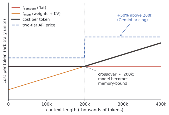
Assuming the crossover is at 200k, you can solve for the model’s KV bytes per token. Setting KV fetch time equal to compute time and cancelling the batch size:

\[\mathrm{bytes}_{\mathrm{tok}} = \frac{\text{mem BW}}{\mathrm{FLOPs}} \cdot \frac{N_{\mathrm{act}}}{\mathrm{len}_{\mathrm{ctx}}} = \frac{1}{300} \cdot \frac{100\mathrm{B}}{200\mathrm{k}} \approx 1.7\ \text{kB per token}\]

Is ~2 kB/token plausible? The KV size is (number of unique attention contexts) × 2 × $d_{\mathrm{head}}$ × (KV heads). With $d_{\mathrm{head}} = 128$ and 8 KV heads and a single global context shared across all layers (the Character AI trick, also used in Gemma), you get exactly 2 kB. Sparse attention gets there with bigger raw numbers divided by the sparsity. So the pricing page is consistent with a real architecture, if maybe a little on the small side.

Input vs output prices

Output tokens cost 3–5x more than input tokens. The two phases differ in tokens per forward pass: decode processes one new token per pass, prefill processes the whole prompt in one pass. Dividing the same roofline by the tokens per pass (len_pass) gives the cost per token: the compute term is flat, and the memory term is a hyperbola that only bites when len_pass is small.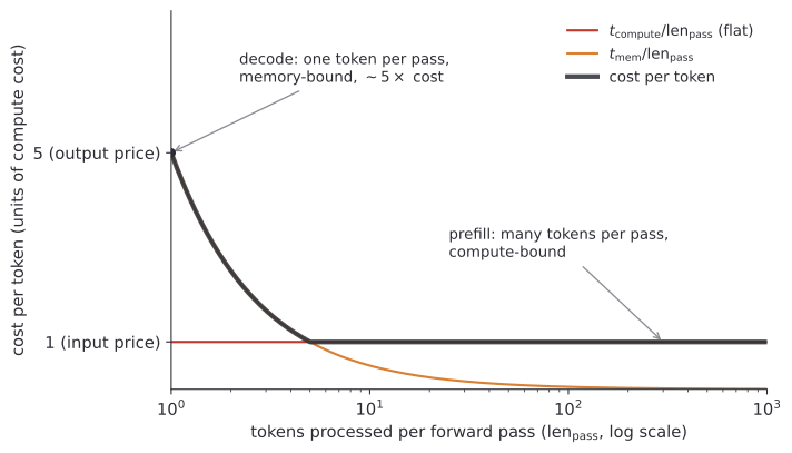

Prefill is compute-bound, decode is memory-bandwidth-bound, and a 5x price gap says decode at the provider’s operating point is deeply memory-bound: they are paying ~5x more per output token in memory time than the compute floor.

This also explains the context length plateau. Contexts jumped from ~8k (GPT-3 era) to 100–200k around GPT-4 and have hovered there for a year or two, which suggests that is the balanced cost point. The barrier to 100M-token contexts (the “in-context learning is enough for AGI” scenario) is memory bandwidth and capacity, and HBM is not getting hugely better. Sparse attention (DeepSeek published one mechanism that effectively puts a square root on the KV term) is a big one-time improvement, but going too sparse costs quality, so it is a get-out, not a solution.

Cache pricing and memory tiers

Providers charge much less for cached input tokens, and charge different rates for keeping a cache alive 5 minutes vs 1 hour. There are two ways to produce a KV cache for a token: rematerialize it from scratch (a forward pass: pure compute cost, nothing to store) or hold it in some memory tier (near-zero retrieval cost, but you occupy capacity that scales with hold time). Each tier down (HBM → host DDR → flash → spinning disk) is cheaper to occupy and slower to retrieve from.

Which tier backs which price? Pope’s rule: a storage tier is well-matched to hold times around its drain time, capacity divided by bandwidth, the same ratio that gave 20 ms for HBM. DDR drains in seconds, flash in about a minute, spinning disk in about an hour. So a 5-minute cache tier and a 1-hour cache tier probably map to flash and spinning disk, which surprised him: “I’m kind of shocked to see spinning disk being used at all.”

Convergent evolution with cryptography

The sit-down portion covers Pope’s blog post on how neural nets and ciphers evolved similar shapes. Both need to thoroughly mix information across all their inputs, and even stirring cake batter alternates directions for the same reason. But they optimize in opposite directions. A neural net is kept differentiable in a useful way: residual connections and LayerNorm exist to keep the derivative simple and meaningful for gradient descent. A cipher is designed so that its derivative is useless: differential cryptanalysis attacks a cipher by differentiating it (over the field of two elements), and a well-designed cipher makes a small input difference blow up into a huge output difference, the avalanche effect. Adversarial examples in image models are exactly the avalanche property showing up where it is not wanted.

Building ciphers out of neural nets is a bad idea (99% of new ciphers get broken), but one construction has productively flowed the other way. A Feistel network turns any non-invertible function $f$ into an invertible two-input block:

\[g(x, y) = (\,y + f(x),\; x\,)\]

To invert, read off $x$ from the second slot, then recover $y = z - f(x)$.

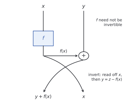
The 2017 RevNets paper imported this into deep learning: make each layer a Feistel block (which turns out to look like a residual connection from two layers back) and the whole network becomes invertible. Training normally has to write every layer’s activations to HBM on the forward pass so that the backward pass can read them, a memory footprint linear in depth and often the largest one in training. An invertible network stores none of it: during the backward pass it undoes the forward pass in lockstep, rematerializing activations as needed.

That is spending compute to save memory, the exact mirror image of the KV cache, which spends memory to save compute. Given where hardware is, the KV cache direction is usually the profitable one, which is a fitting last word for a lecture that is mostly about the price of memory.