In [lecture](http://www1.mate.polimi.it/~antonietti/PERSONAL_WEBPAGE/Teaching_files/Antonietti_DGintro_2.pdf)
[notes](http://sanum.github.io/2016/slides/Reddy.pdf)
related to the
[Discontinuous Galerkin method](https://en.wikipedia.org/wiki/Discontinuous_Galerkin_method),
there is
mention of a *magic formula* which AFAIK first appeared on a paper[^arnold82] by
Douglas Arnold (at least in this context).
It has been proven and all, but it's still called magic because its reasoning is
not apparent at first glance. The magic formula is actually a superset of
the divergence theorem, generalized to discontinuous fields. But to make that
generalization, we need to abandon the standard formulation which starts by
creating a triangular mesh, and consider arbitrary partitionings of a domain.
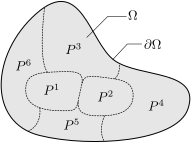
A domain $\Omega$ is partitioned into parts $P^i$, $i=1,\dots,n$ as follows:
$$\Omega=\bigcup_{i=1}^{n} P^i$$
$$\mathcal{P} = \{P^1,\dots,P^{n}\}$$
We call the set of parts $\mathcal{P}$ a **partition** of $\Omega$.
# Broken Hilbert Spaces
We allow the vector field $\boldsymbol{u}$ to be **discontinuous at
boundaries** $\partial P^i$ and **continuous in** $P^i$, $i=1,\dots,n$.
To this end, we define the **broken Hilbert
space** over partition $\mathcal{P}$
$$\begin{equation}
H^m(\mathcal{P}) := \{\boldsymbol{v}\in L^2(\Omega)^{n_d} \mid \forall P\in\mathcal{P}, \boldsymbol{v}|_P \in H^m(P)\}
\end{equation}$$
It can be seen that $H^m(\mathcal{P})\subseteq H^m(\Omega)$.
# Part Boundaries
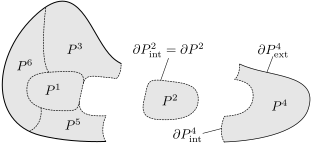
Topologically, a part may share boundary with $\Omega$, like $P^4$.
In that case, the boundary of the part is divided into an
**interior** boundary and **exterior** boundary:
$$\begin{equation}
\partial P_{\text{ext}}^i = \partial P^i \cap \partial\Omega
\quad\text{and}\quad
\partial P_{\text{int}}^i = \partial P^i \setminus \partial P_{\text{ext}}^i
\end{equation}$$
If a part has an exterior boundary, it is said to be an **external** part
($P^3$, $P^4$, $P^5$, $P^6$). If it
does not have any exterior boundary, it is said to be an **internal**
part.($P^1$, $P^2$).
# Divergence theorem over parts
For a vector field $\boldsymbol{v}\in H^1(\mathcal{P})$,
$i=1,\dots,n$, we can write the following integral as a sum and apply the
divergence theorem afterward
$$\begin{equation}
\begin{aligned}
\int_\Omega \div{\boldsymbol{v}} \,dV
&= \sum\limits_{i=1}^{n}\int_{P^i}\div\boldsymbol{v} \,dV
= \sum\limits_{i=1}^{n}\int_{\partial P^i} \boldsymbol{v}\cdot\boldsymbol{n} \,dA \\
&= \sum\limits_{i=1}^{n}\int_{\partial P_{\text{ext}}^i} \boldsymbol{v}\cdot\boldsymbol{n} \,dA
+\sum\limits_{i=1}^{n}\int_{\partial P_{\text{int}}^i} \boldsymbol{v}\cdot\boldsymbol{n} \,dA
\end{aligned}
\end{equation}$$
We define the portion $\Gamma^{ij}$ of the boundary that part
$P^i$ shares with $P^j$ as the **interface** between $P^i$ and $P^j$.
$$\begin{equation}
\Gamma^{ij} = \partial P^i \cap \partial P^j
\end{equation}$$
If $P^i$ and $P^j$ are not neighbors, we simply have $\Gamma^{ij}=\emptyset$.
# Integrals over interior boundaries
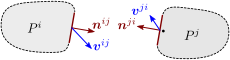
For opposing parts $P^i$ and $P^j$,
we have different values of the function $\boldsymbol{v}^{ij} = \boldsymbol{v}|_{\Gamma^{ij}}$
and conjugate normal vectors at the
interface $\Gamma^{ij}$:
$$\begin{equation}
\boldsymbol{v}^{ij}\neq\boldsymbol{v}^{ji}
\quad\text{and}\quad
\boldsymbol{n}^{ij} = -\boldsymbol{n}^{ji}
\end{equation}$$
Since
$$\begin{equation}
\partial P_{\text{int}}^i
= \bigcup_{j=1}^{n} \Gamma^{ij}
\quad \text{for}\quad i=1,\dots,n
\end{equation}$$
we can rearrange the integral over interior boundaries as
$$\begin{equation}
\sum\limits_{i=1}^{n}\int_{\partial P_{\text{int}}^i} \boldsymbol{v}\cdot\boldsymbol{n} \,dA
= \sum\limits_{i=1}^{n}\sum\limits_{j=1}^{n}\int_{\Gamma^{ij}} \boldsymbol{v}^{ij}\cdot\boldsymbol{n}^{ij} \,dA
\end{equation}$$
# The jump operator
Integrals over the same interface can be grouped together:
$$\begin{equation}
\sum\limits_{i=1}^{n}\sum\limits_{j=1}^{n}\int_{\Gamma^{ij}} \boldsymbol{v}^{ij}\cdot\boldsymbol{n}^{ij} \,dA
=
\sum\limits_{i=1}^{n}\sum\limits_{j=i}^{n}\int_{\Gamma^{ij}\equiv\Gamma^{ji}}
(\boldsymbol{v}^{ij}\cdot\boldsymbol{n}^{ij} + \boldsymbol{v}^{ji}\cdot\boldsymbol{n}^{ji}) \,dA
\end{equation}$$
Defining the **jump** of $\boldsymbol{v}$ across $\Gamma^{ij}$
$$\begin{equation}
\llbracket\boldsymbol{v}\rrbracket_{\Gamma^{ij}} = \boldsymbol{v}^{ij} - \boldsymbol{v}^{ji}
\end{equation}$$
The jump of a function measures its discontinuity across interfaces.
We can write
$$\begin{equation}
\int_{\Gamma^{ij}} \llbracket\boldsymbol{v}\rrbracket_{\Gamma^{ij}}\cdot\boldsymbol{n}^{ij} \,dA
= \int_{\Gamma^{ij}} (\boldsymbol{v}^{ij}\cdot\boldsymbol{n}^{ij} + \boldsymbol{v}^{ji}\cdot\boldsymbol{n}^{ji}) \,dA
\end{equation}$$
We may drop the superscripts where there is no confusion.
# Interfaces and external boundaries
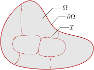
It is convenient to group the interfaces:
$$\begin{equation}
\boxed{
\mathcal{I} := \{\Gamma^{ij}\mid i=1,\dots,n; j=i,\dots,n\}
}
\end{equation}$$
which allows us to write
$$\begin{equation}
\sum\limits_{i=1}^{n}\sum\limits_{j=i}^{n}
\int_{\Gamma^{ij}} \llbracket\boldsymbol{v}\rrbracket\cdot\boldsymbol{n} \,dA
= \sum\limits_{\Gamma\in\mathcal{I}} \int_{\Gamma} \llbracket\boldsymbol{v}\rrbracket\cdot\boldsymbol{n}\,dA
\end{equation}$$
It's obvious that the union of part external boundaries equals the domain boundary:
$$\begin{equation}
\bigcup_{i=1}^{n} \partial P_{\text{ext}}^i = \partial \Omega
\end{equation}$$
which allows us to write
$$\begin{equation}
\sum\limits_{i=1}^{n}\int_{\partial P_{\text{ext}}^i} \boldsymbol{v}\cdot\boldsymbol{n} \,dA
= \int_{\partial\Omega} \boldsymbol{v}\cdot\boldsymbol{n} \,dA
\end{equation}$$
With the results obtained, we put forward a **generalized** version of the divergence
theorem: Let $\boldsymbol{v}\in H^1(\mathcal{P})$ be a vector field. Then we have
$$\begin{equation}
\boxed{
\int_\Omega \div\boldsymbol{v} \,dV
= \int_{\partial\Omega} \boldsymbol{v}\cdot\boldsymbol{n} \,dA
+ \sum\limits_{\Gamma\in\mathcal{I}} \int_{\Gamma} \llbracket\boldsymbol{v}\rrbracket\cdot\boldsymbol{n} \,dA
}
\end{equation}$$
Verbally,
the **integral of the divergence of a vector field over a domain** $\Omega$
equals
**its integral over the domain boundary** $\partial\Omega$,
plus
the **integral of its jump over part interfaces** $\mathcal{I}$.
In the case of a **continuous field**, the jumps **vanish** and this
reduces to the regular divergence theorem.
# The Magic Formula
There are different versions of the magic formula for scalar, vector and tensor
fields, and for different IBVPs. I won't try to derive them all, but give an
example: If we were substitute a linear mapping
$\boldsymbol{A}\boldsymbol{v}$
instead of $\boldsymbol{v}$, we would have the jump
$\llbracket \boldsymbol{A}\boldsymbol{v} \rrbracket$ on the right-hand side.
We introduce the vector and tensor **average** operator $$\{\cdot\}$$
$$\begin{equation}
\{\boldsymbol{v}\}_{\Gamma^{ij}} = \frac{1}{2} (\boldsymbol{v}^{ij} + \boldsymbol{v}^{ji})
\quad\text{and}\quad
\{\boldsymbol{A}\}_{\Gamma^{ij}} = \frac{1}{2} (\boldsymbol{A}^{ij} + \boldsymbol{A}^{ji})
\end{equation}$$
and **tensor jump** operator
$\llbracket\cdot\rrbracket$
$$\begin{equation}
\llbracket\boldsymbol{A}\rrbracket_{\Gamma^{ij}} = \boldsymbol{A}^{ij} - \boldsymbol{A}^{ji}
\end{equation}$$
We also note the boundary jump/average property which is used on the integral
over $\partial\Omega$
$$\begin{equation}
\boxed{
\{\boldsymbol{v}\} = \llbracket\boldsymbol{v}\rrbracket = \boldsymbol{v}
\quad \text{on}\quad\partial\Omega
}
\label{eq:property1}
\end{equation}$$
(**This property is used implicitly in many places, and often causes confusion**).
These definitions allow us to write the identity
$$\begin{equation}
\boxed{
\llbracket\boldsymbol{A}\boldsymbol{v}\rrbracket = \llbracket\boldsymbol{A}\rrbracket\{\boldsymbol{v}\} + \{\boldsymbol{A}\}\llbracket\boldsymbol{v}\rrbracket
}
\end{equation}$$
which is easily proven when expanded.
The different versions of the magic formula are obtained by
substituting the identities above---or their analogs---in the discontinuous
divergence theorem.
[^arnold82]: Douglas N. Arnold. An interior penalty finite element method with discontinuous elements. SIAM J. Numer. Anal., 19(4):742--760, 1982.